Finding transition states with NEB-TS
Suppose you wanted to predict the transition state (TS) for the hydrolysis of methyl-acetate into acetic acid and methanol:
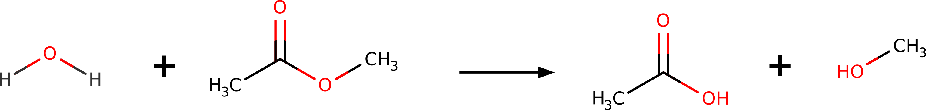
Maybe you need to investigate the mechanism, or even to compute the \(\Delta G^\dagger\) and try to predict reaction rates. How could one do that using theory?
In ORCA there is a black box method called NEB-TS (from Nudged Elastic Band with TS optimization), that can find the TS structure only from the geometries of the reactants and products!
Defining your reactants and products
So the first step is to optimize the "reactants" and "products". Please, have in mind that here it means everything that is left and right of the arrow, the collection of molecules. First, for the reactant, after drawing the initial guess and doing a Geometry optimization using:
!B3LYP DEF2-SVP OPT D4
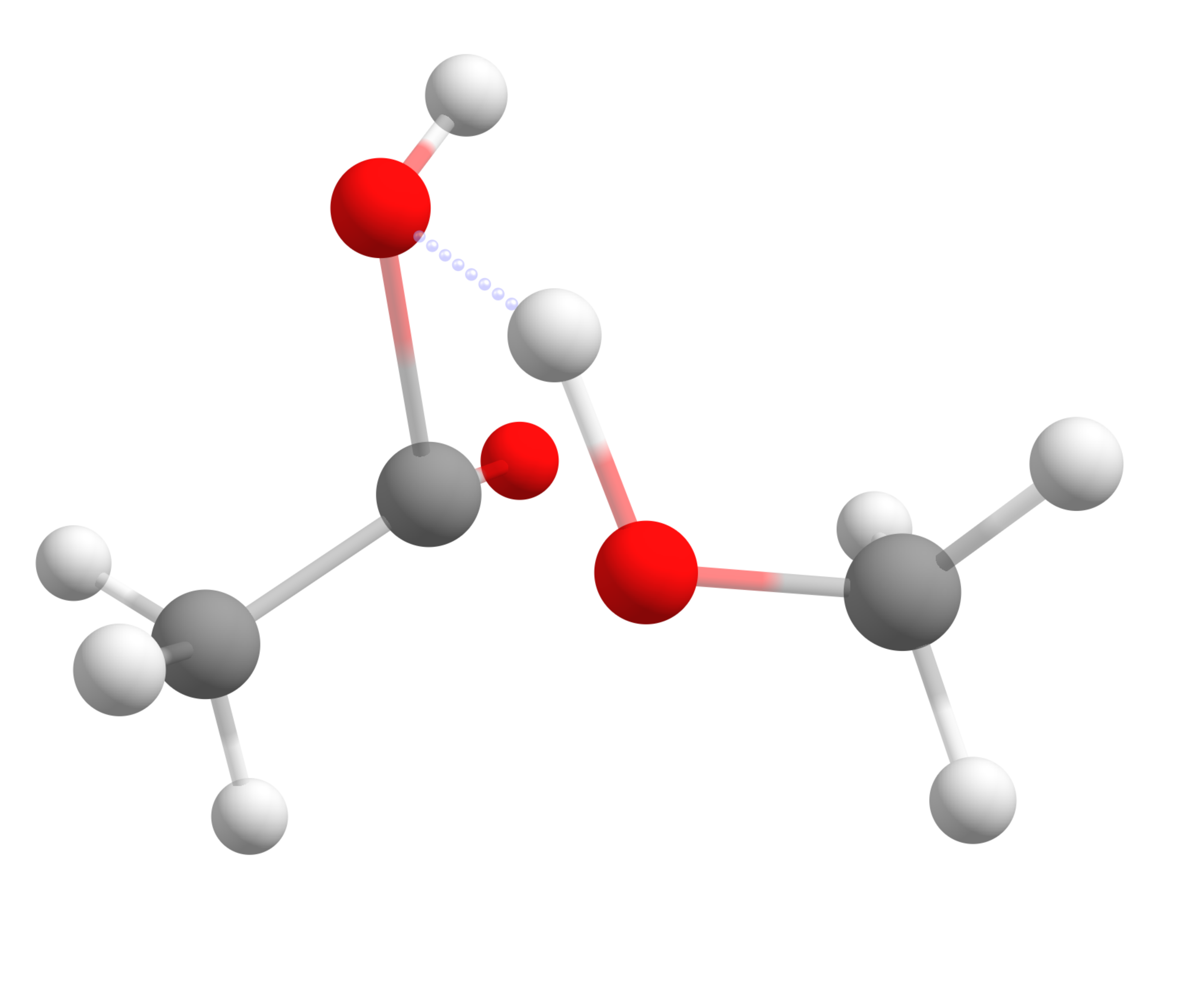
one gets, for instance, the following geometry:
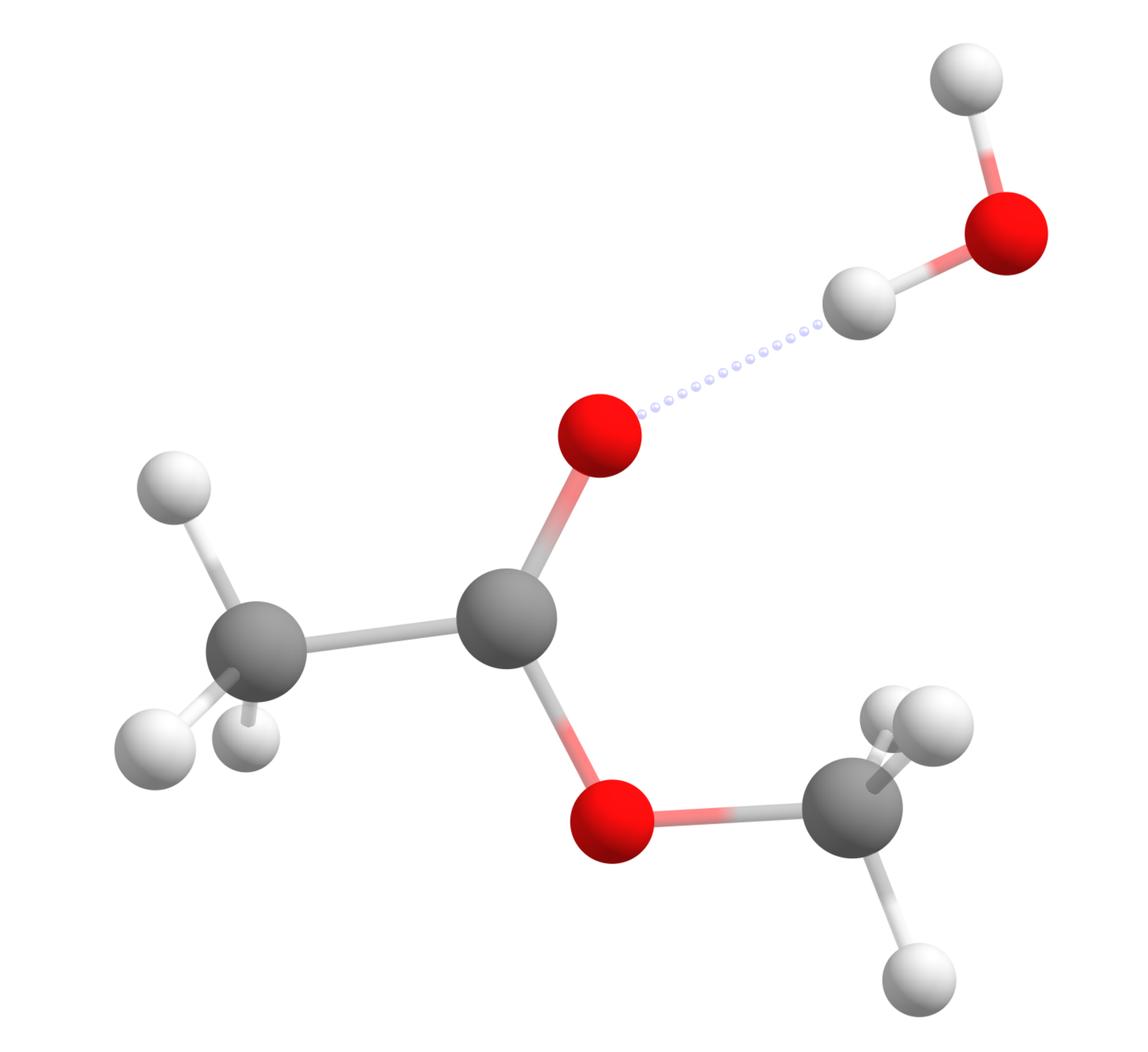
with the nucleophilic water making a hydrogen bond with the carbonyl group. Rearranging the atoms to make a guess product structure, and after optimizing with the same method, one gets:
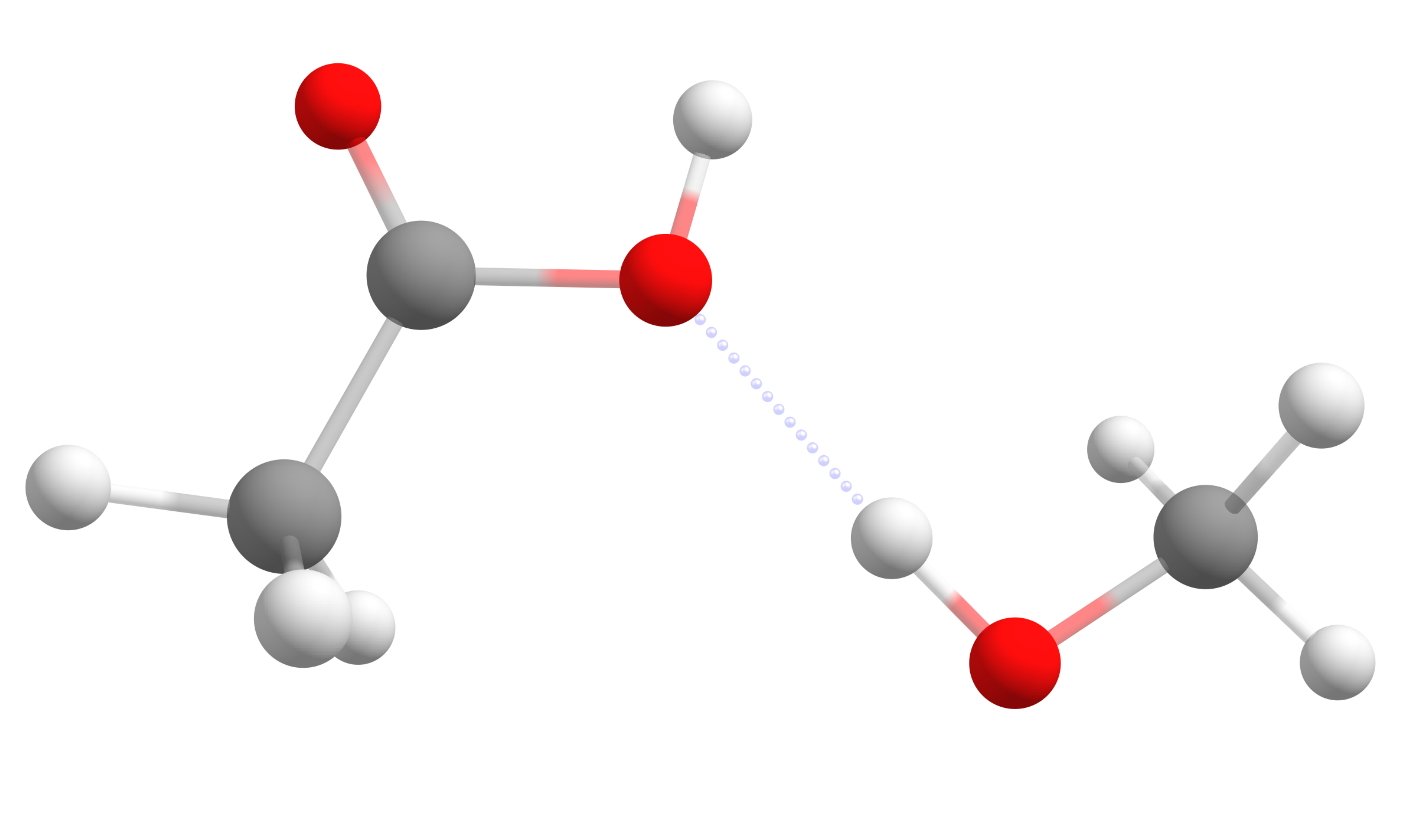
and we are ready to find the transition state.
Important
In order for the NEB-TS to work, the atom numbering in both reactant and product geometries must be the same. Which means that a given carbon on the reactant, should have the same order in the xyz table in the product. The best way to guarantee this is to start from one geometry, make a copy and move the atoms to draw the next structure.
Note
If using Avogadro, you have to disable the Adjust Hydrogen feature, otherwise atoms will be automatically placed when a bond is broken, and not necessarily where you want them to be.
Note
The idea is not to optimize all molecules separately and just join then in a single file, but rather already build your "reactant" and "product" adducts in a certain orientation that makes sense with respect to the expected reaction, like done in the example.
Making the NEB-TS input
The NEB-TS input is quite simple, one has to add only NEB-TS in the main input, and give the name of the product xyz file on the %NEB options:
!B3LYP DEF2-SVP D4 NEB-TS FREQ
%NEB NEB_END_XYZFILE "product.xyz" END
* XYZfile 0 1 reactant.xyz
In case you have a guess structure for the TS as well, that can be included as:
!B3LYP DEF2-SVP D4 NEB-TS FREQ
%NEB NEB_END_XYZFILE "product.xyz"
     NEB_TS_XYZFILE "guessTS.xyz"
END
* XYZfile 0 1 reactant.xyz
and you can already run it.
Note
The reactant and products will not be optimized during the default run, so make sure you are using the same method you chose for the previous optimization. If you want to reoptimize them, set PREOPT_ENDS TRUE under %NEB.
Running the NEB
After the calculation starts, the first output is:
----------------------
NEB settings
----------------------
Method type                             ....  climbing image
Threshold for climbing image            ....  2.00e-02 Eh/Bohr
Free endpoints                          ....  off
Tangent type                            ....  improved
Number of intermediate images           ....  8
Number of images free to move           ....  8
Spring type for image distribution      ....  distance between adjacent images
Spring constant                         ....  energy weighted (0.0100 -to- 0.1000) Eh/Bohr^2
Spring force perp. to the path          ....  none
Generation of initial path              ....  image dependent pair potential
Initial path via TS guess               ....  off
[...]
which contains some details of the method. Then, comes the construction of a initial path:
Generation of  the initial path:
Minimize RMSD between reactant and product configurations     .... done
       RMSD before minimization         ....  2.1153 Bohr
       RMSD after minimization          ....  1.6611 Bohr
Performing linear interpolation         ....  done
Interpolation using                     ....  IDPP (Image Dependent Pair Potential)
IDPP-Settings:
       Remove global transl. and rot.   ...   true
       Convergence tolerance            ....  0.0100 1/Ang.^3
       Max. numer of iterations         ....    7000
       Spring constant                  ....  1.0000 1/Ang.^4
       Time step                        ....  0.0100 fs
       Max. movement per iteration      ....  0.0500 Ang.
       Full print                       ....  false
idpp initial path generation successfully converged in 117 iterations
Displacement along initial path:             11.6511 Bohr
Writing initial trajectory to file      ....  NEBTS_initial_path_trj.xyz
The idea here is to use a method called IDPP to create a series of images, from the reactant to products, that will be optimized together using the NEB formalism.
The initial path is saved in basename_initial_path_trj.xyz, and it is recommended to check if that makes sense. In this case, we get the following sequence of eight "images":
which looks reasonable, with the proton being transferred from the water to the methanol as it leaves.
Note
Trajectory files are simply multixyz files containing several structures one after the other. Chemcraft, Molden and some other software can open those directly. Avogadro requires going to "Extensions" -> "Animation..." and the file can be opened and even animated.
Then, the iterative process starts:
Starting iterations:

Optim.  Iteration  HEI  E(HEI)-E(0)  max(|Fp|)   RMS(Fp)    dS
Switch-on CI threshold               0.020000
   LBFGS     0      5    0.297110    0.116137   0.026058  11.6511
   LBFGS     1      5    0.277441    0.092448   0.021661  11.5993
   LBFGS     2      6    0.262453    0.111904   0.022265  11.5925
   LBFGS     3      6    0.252519    0.082144   0.017474  11.6060
and after some convergence, a "climbing image" (CI) is found:
Image  6 will be converted to a climbing image in the next iteration (max(|Fp|) < 0.0200)

Optim.  Iteration  CI   E(CI)-E(0)   max(|Fp|)   RMS(Fp)    dS     max(|FCI|)   RMS(FCI)
Convergence thresholds               0.020000   0.010000            0.002000    0.001000
   LBFGS    23      6    0.160709    0.029259   0.004374  12.8932    0.030101    0.007764
   LBFGS    24      6    0.159481    0.051391   0.006905  13.0230    0.054092    0.012911
   LBFGS    25      6    0.156310    0.068675   0.009114  13.3077    0.072840    0.017253
   LBFGS    26      6    0.153131    0.031865   0.004433  13.3046    0.031225    0.007908
This is our first guess to the TS final structure.
Optimization of the TS
After some iterations, the NEB-CI converges:
                                .--------------------.
          ----------------------| CI-NEB convergence |-------------------------
          Item                value                   Tolerance       Converged
          ---------------------------------------------------------------------
          RMS(Fp)             0.0006879134            0.0100000000      YES
          MAX(|Fp|)           0.0032907070            0.0200000000      YES
          RMS(FCI)            0.0006591030            0.0010000000      YES
          MAX(|FCI|)          0.0016597640            0.0020000000      YES
          ---------------------------------------------------------------------

The elastic band and climbing image have converged successfully to a MEP in 128 iterations!

                    *********************H U R R A Y*********************
                    ***        THE NEB OPTIMIZATION HAS CONVERGED     ***
                    *****************************************************
and a transition state optimization starts. First, a guess Hessian matrix is built using information from the previous NEB and a saddle point search is initiated.
If the TS is fully optimized, a summary for the whole NEB-TS is printed:
            ***********************HURRAY************************
            ***        THE TS OPTIMIZATION HAS CONVERGED      ***
            *****************************************************

---------------------------------------------------------------
                      PATH SUMMARY FOR NEB-TS
---------------------------------------------------------------
All forces in Eh/Bohr. Global forces for TS.

Image     E(Eh)   dE(kcal/mol)  max(|Fp|)  RMS(Fp)
  0     0.000    -344.38971      0.00       0.00014   0.00003
  1     2.024    -344.38507      2.91       0.00144   0.00053
  2     3.395    -344.38062      5.70       0.00150   0.00055
  3     4.863    -344.38237      4.61       0.00167   0.00064
  4     5.663    -344.36742     13.98       0.00329   0.00102
  5     6.043    -344.33717     32.97       0.00274   0.00097
  6     6.336    -344.32049     43.44       0.00178   0.00058 <= CI
  7     6.754    -344.34916     25.45       0.00260   0.00098
  8     7.426    -344.38096      5.49       0.00143   0.00058
  9     9.661    -344.38666      1.91       0.00023   0.00007
and the frequencies of the TS are computed, to verify if that has only one negative frequency. The result for this case is:
-----------------------
VIBRATIONAL FREQUENCIES
-----------------------

Scaling factor for frequencies =  1.000000000  (already applied!)

   0:         0.00 cm**-1
   1:         0.00 cm**-1
   2:         0.00 cm**-1
   3:         0.00 cm**-1
   4:         0.00 cm**-1
   5:         0.00 cm**-1
   6:     -1149.57 cm**-1 ***imaginary mode***
   7:       106.27 cm**-1
   8:       135.34 cm**-1
   9:       188.41 cm**-1
proving that the optimized TS structure is indeed a saddle point.
The final trajectory from the reactants to products can be read from basename_MEP_trj.xyz, and the final transition state geometry, saved in basename_NEB-TS_converged.xyz is:
One can see that the TS has a tetrahedral carbon atom, as expected from the experimental mechanism, and there is a concerted transfer of proton to the leaving methoxy group.
Note
This calculation was run in gas phase to simplify the explanation. If one includes the solvent, the mechanism will be more complex and the proton transfer can occur, possibly, through an external water molecule.
Possible intermediates
During the NEB-CI process, the following message could appear:
Possible intermediate minimum found at image(s): 7
  => have a look at the .interp file.
  => it is often a good idea to divide the path calculation into smaller fragments.
That was because a local minimum was detected along the reaction path. Actually, there could be even more than one.
The energies following the reaction minimum energy path are printed in the "interp" files and can be plotted to have a better look at it:
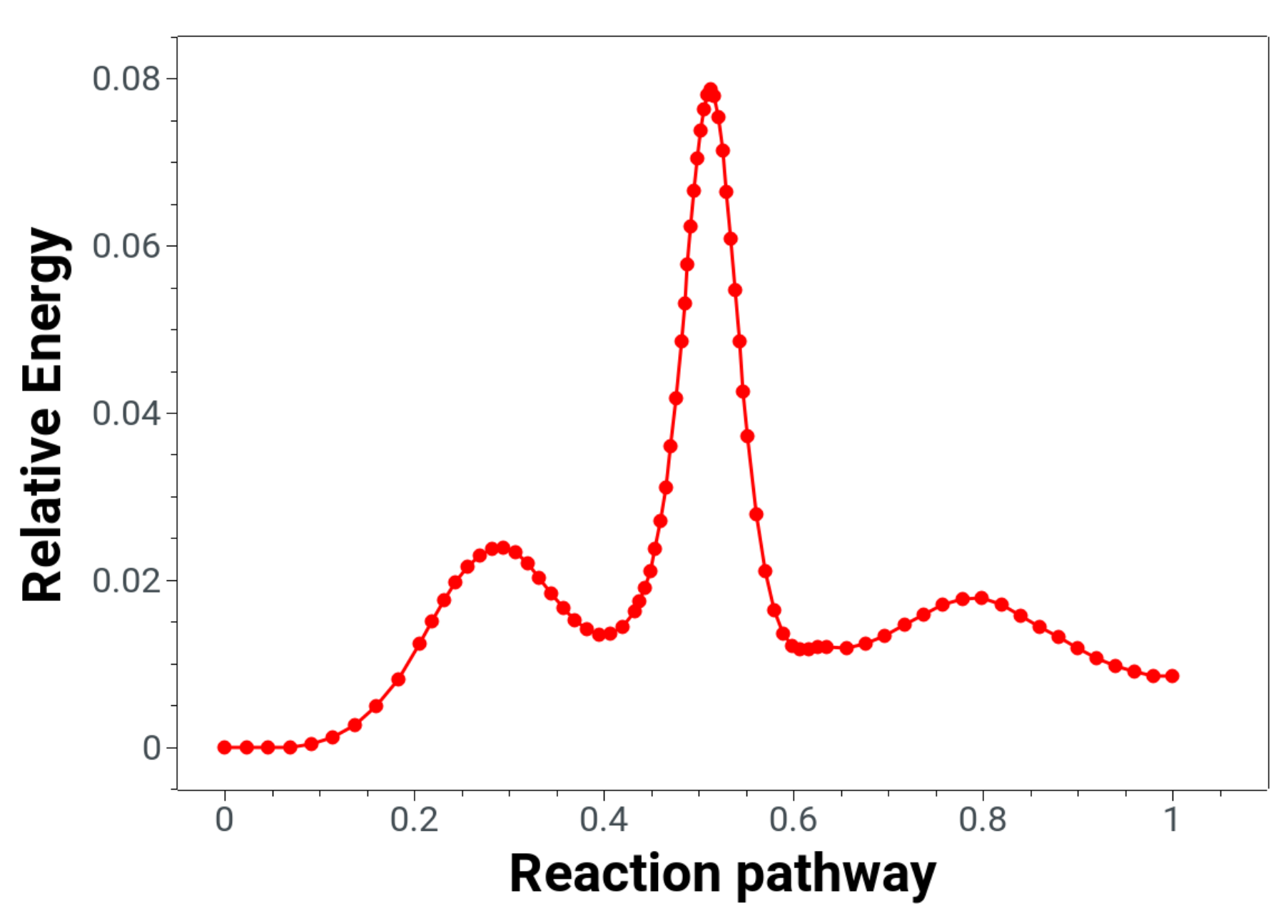
Here one clearly sees that there are two intermediates and one should optimize this structures as well in order to predict reaction energies correctly, and maybe rerun the NEB-TS with these new rectant and product guesses.
Starting structures
Reactant
C         -3.84500       -0.17571       -0.03921
C         -2.44492        0.32082        0.15466
H         -4.02399       -1.04086        0.60409
H         -4.00401       -0.43615       -1.08861
H         -4.55059        0.61392        0.23466
O         -1.55509       -0.65188       -0.18018
C         -0.18433       -0.27497       -0.02916
H          0.05373        0.57033       -0.68208
H          0.43501       -1.12619       -0.32499
H          0.03294       -0.03494        1.01615
O         -2.15827        1.44183        0.55653
O         -0.06767        3.07881        1.16647
H         -0.50923        3.90074        1.42789
H         -0.83167        2.50085        0.95538
Product
C         -3.44596       -0.05388        0.06874
C         -2.45275        1.00891        0.40403
H         -3.34585       -0.89157        0.76374
H         -3.29683       -0.38937       -0.95986
H         -4.45598        0.35325        0.17275
O          0.13193       -1.79894       -0.30248
C          1.49893       -1.43301       -0.26662
H          1.66462       -0.57388       -0.92141
H          2.10288       -2.27456       -0.61417
H          1.78363       -1.18238        0.75829
O         -2.67152        2.20314        0.50109
O         -1.20490        0.52554        0.57750
H         -0.69584        1.33651        0.80013
H         -0.37607       -1.03530        0.03854