Infrared and Raman
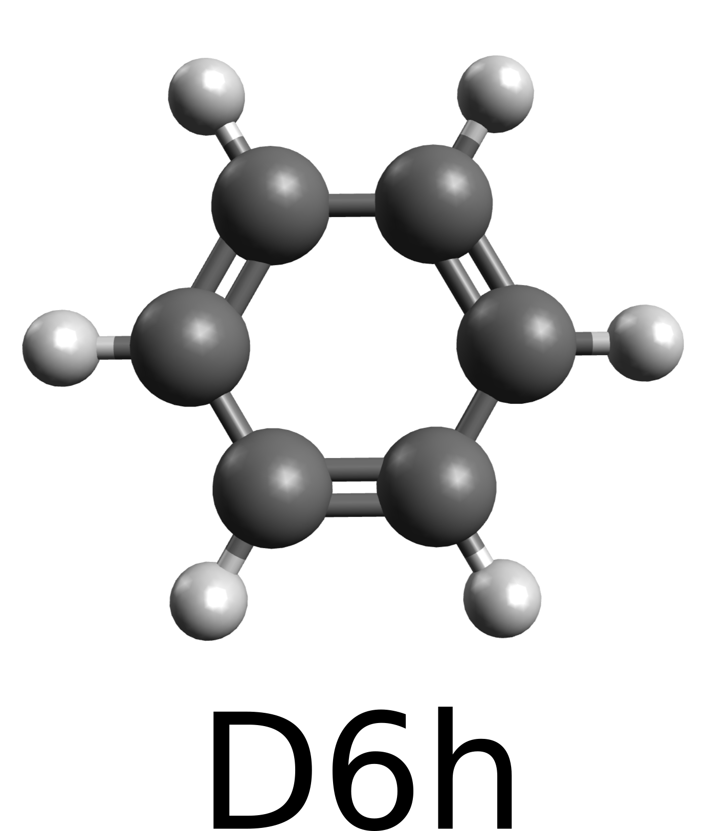
The prediction of infrared (IR) and (non-resnonant) Raman spectra are nowadays a straightforward task in computational chemistry. Let us use ORCA to predict the fundamental frequencies and intensities for benzene.
Because of its symmetry, the selection rules predict that these bands are mutually exclusive, with \(A_{2u}\) and \(E_{1u}\) modes being the most IR active (\(B_{1u}, B_{2u}\) and \(E_{2u}\) modes are less intense), while the \(A_{1g}, E_{1g}\) and \(E_{2g}\) are Raman active. For comparison, the complete set of experimental values can be found on NIST's website.
Predicting infrared spectra
Assuming you have already done a Geometry optimization, you can get the infrared spectrum of any molecule by running a frequency calculation, e.g. with DFT:
!BP86 DEF2-SVP OPT FREQ
* xyzFILE 0 1 ben_D6h.xyz
or for any method without the analytic Hessian using !NUMFREQ:
!B2PLYP DEF2-SVP OPT NUMFREQ
* xyzFILE 0 1 ben_D6h.xyz
and the vibrational frequencies will be printed:
-----------------------
VIBRATIONAL FREQUENCIES
-----------------------

Scaling factor for frequencies =  1.000000000  (already applied!)

   0:         0.00 cm**-1
   1:         0.00 cm**-1
   2:         0.00 cm**-1
   3:         0.00 cm**-1
   4:         0.00 cm**-1
   5:         0.00 cm**-1
   6:       401.59 cm**-1
   7:       401.64 cm**-1
   8:       600.33 cm**-1
   9:       600.37 cm**-1
   [...]
followed by the vibrational modes and the:
-----------
IR SPECTRUM
-----------

 Mode   freq       eps      Int      T**2         TX        TY        TZ
       cm**-1   L/(mol*cm) km/mol    a.u.
----------------------------------------------------------------------------
  6:    401.59   0.000000    0.00  0.000000  (-0.000000 -0.000000 -0.000088)
  7:    401.64   0.000000    0.00  0.000000  (-0.000000  0.000000  0.000000)
  8:    600.33   0.000000    0.00  0.000000  (-0.000000 -0.000000 -0.000000)
  9:    600.37   0.000000    0.00  0.000000  (-0.000000  0.000000 -0.000000)
 10:    668.72   0.016625   84.02  0.007758  ( 0.000000 -0.000000 -0.088082)
  [...]
where the dipole derivatives necessary to compute the IR intensities are printed after each frequency.
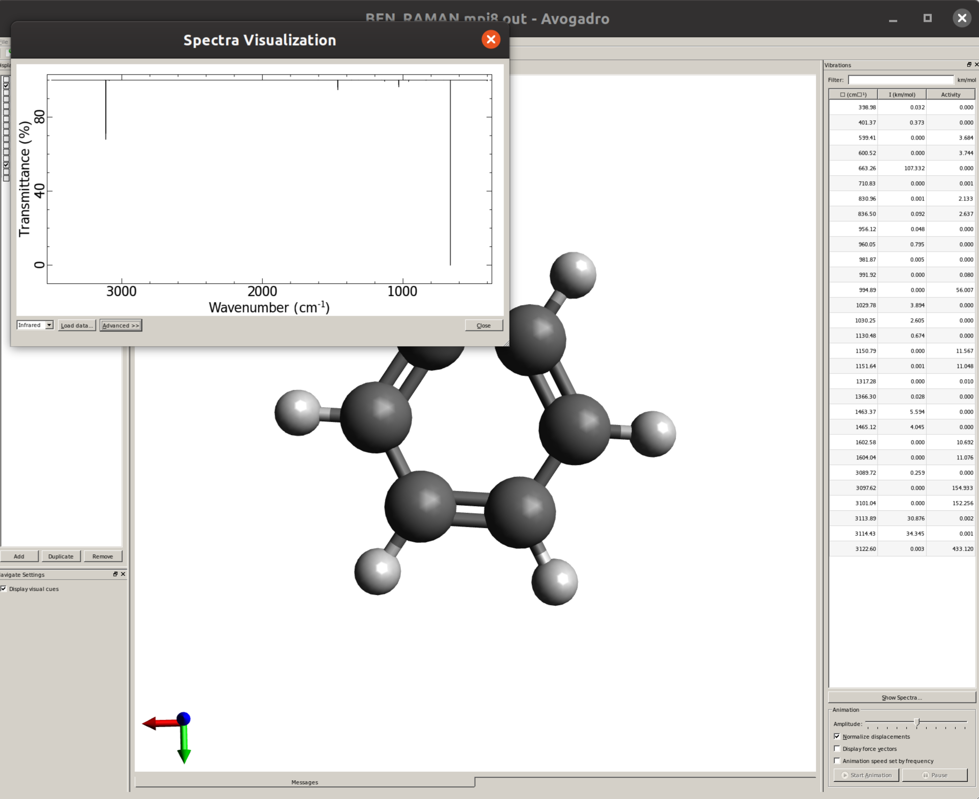
Plotting the IR spectrum
The IR spectrum can then be immediately generated Using Avogadro as a GUI. Just open the saved output file and click on "Show Spectra..." to open a new window were the graphic will be plotted:
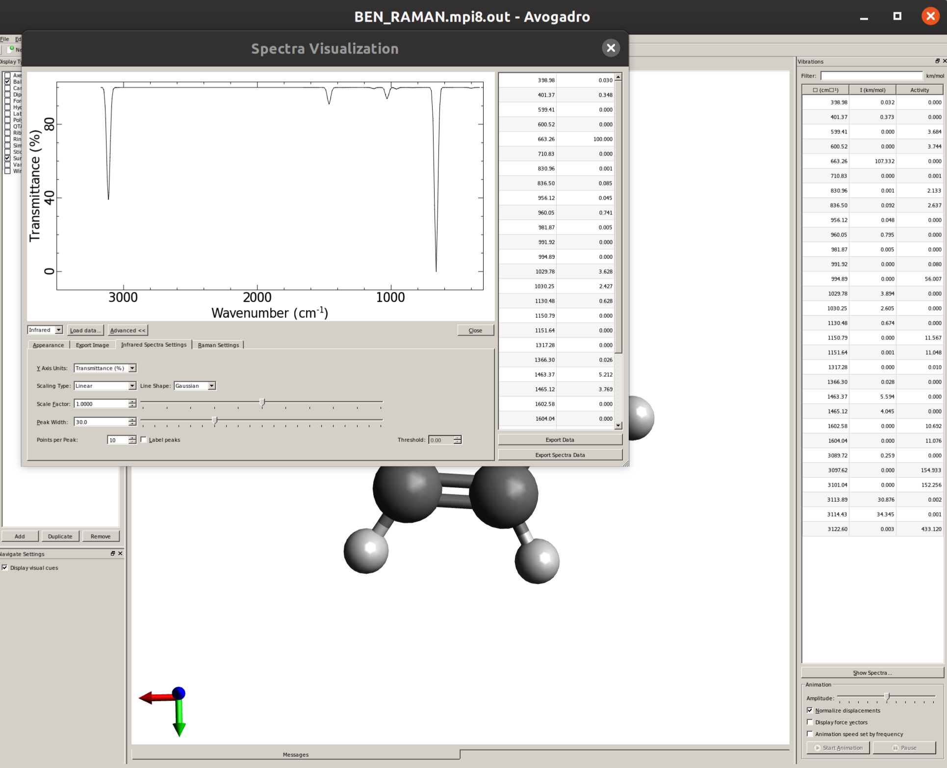
By default, only thin lines corresponding to each frequency are printed. In order to make your predicted spectra look more like an experimental one, some line broadening is needed. This can be easily done by clicking in "Advanced >>", and then on the "Infrared Spectra Settings" tab the "Peak Width" can be set, say to \(30 cm^{-1}\), resulting in a spectrum like:
Visualizing modes
In order to have a better assignment of the IR peaks, one can click on the corresponding frequency in the main Avogadro window and then on "Start Animation" to make a small movie of the mode displacement.
As an example, if one chooses the \(A_{2u}\) IR active mode at \(668 cm^{-1}\), that in textbooks is commonly assigned as an out-of-plane C-H bending, one gets:
exactly as expected. The symmetry breaking creates a temporary dipole one the benzene molecule, and that allows for intensity on a IR transition.
Note
The line broadening must be included ad hoc here because it is related to the lifetimes of vibrational excited states and structural parameters that were not accounted for in the calculation and might vary depending on the experimental conditions.
Important
Be aware that we are predicting only fundamental transitions, so no overtones and combination bands are included!
Here is a table comparing the calculated and experimental values for the IR fundamentals:
Mode |
Experiment |
Predicted |
|---|---|---|
\(E_{2u}\) Ring deform |
410 |
401 |
\(A_{2u}\) C-H bend |
673 |
668 |
\(B_{1u}\) Ring deform |
1010 |
961 |
\(E_{1u}\) C-H bend |
1038 |
1031 |
\(B_{2u}\) C-H bend |
1150 |
1130 |
\(E_{1u}\) C=C str |
1486 |
1462 |
\(B_{1u}\) C-H str |
3068 |
3092 |
\(E_{1u}\) C-H str |
3063 |
3116 |
Predicting Raman spectra
In a similar way, the non-resonant Raman spectra composed of fundamental transitions can be predicted. The main difference here is that the derivatives of the polarizability have to be computed numerically, so that the !NUMFREQ flag has to be used, together with a keyword under %ELPROP to request the calculation of polarizabilties:
!BP86 DEF2-SVP NUMFREQ
%ELPROP
   POLAR 1
END
* xyzFILE 0 1 ben_optimized.xyz
Here POLAR 1 means that the polarizability is computed analytically, by solving the CP-SCF equations. However, this option is only available for regular DFT and HF. For other methods, POLAR 2 can be chosen to compute it directly from the derivatives of the dipole moment. Please check the ORCA manual for all available options.
If everything runs without errors, one should also see now, after the "IR SPECTRUM" section, the:
--------------
RAMAN SPECTRUM
--------------

 Mode    freq (cm**-1)   Activity   Depolarization
-------------------------------------------------------------------
   6:       402.42      0.000000      0.333796
   7:       402.52      0.000000      0.697141
   8:       599.57      3.620435      0.750000
   9:       600.01      3.689274      0.749930
  10:       668.85      0.000000      0.345574
  11:       711.92      0.000001      0.749987
  12:       838.57      2.715404      0.750000
  [...]
It is important to say the Raman intensities are a more complicated subject than those of IR and are much more dependent on the experimental setup, that is why we print here the so-called "Raman Activity" instead [Hess2002], because it is setup invariant.
Plotting the Raman spectrum
Again using Avogadro, one can easily generate the spectrum by opening the output file, clicking on "Show Spectra ..." and then selecting "Raman" on the drop down menu on the left:
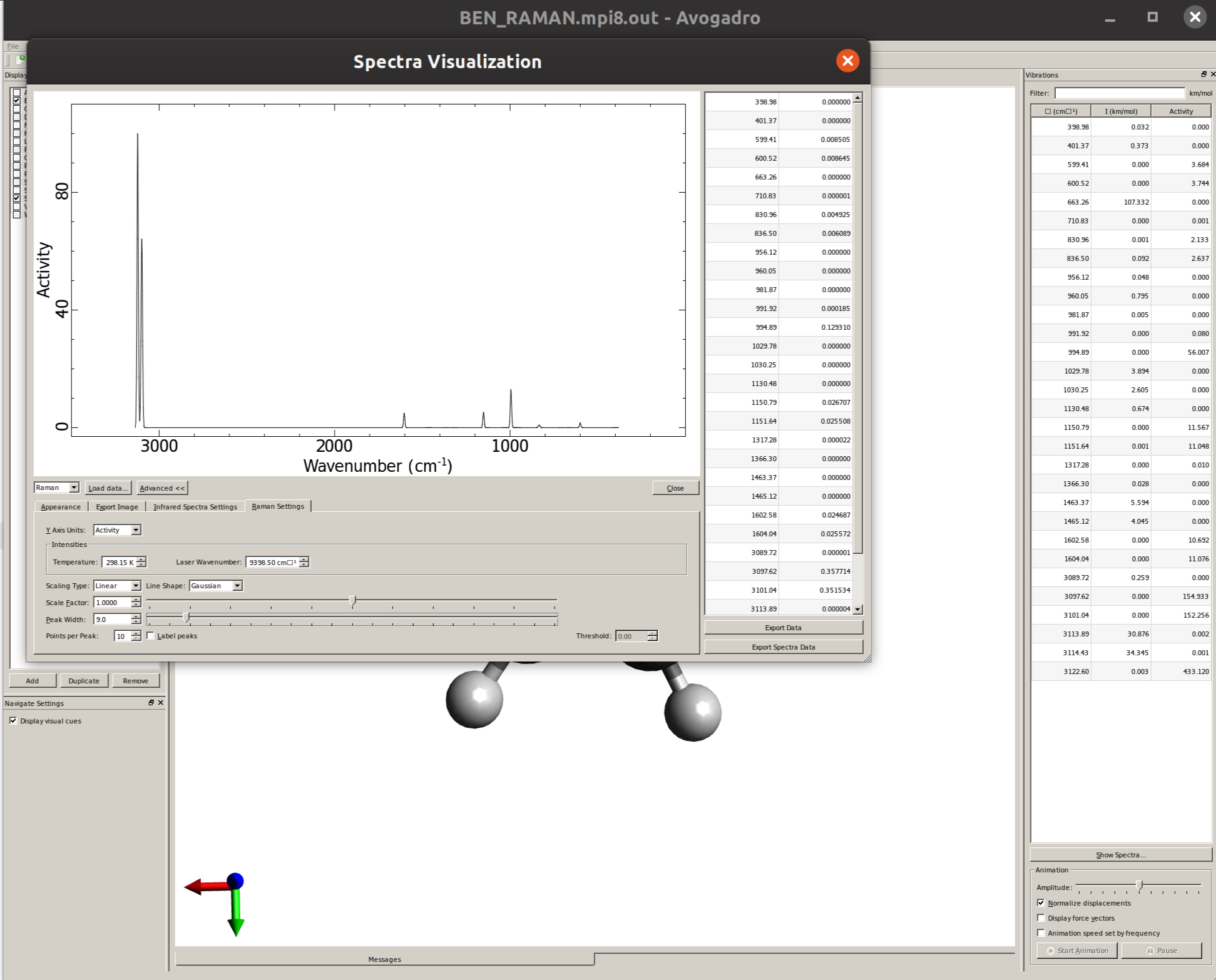
The "Raman Settings" tab now contains the options to shift frequencies and define a line width.
Again, we can compile a table comparing the calculated and experimental values for the Raman fundamentals:
Mode |
Experiment |
Predicted |
|---|---|---|
\(E_{2g}\) Ring deform |
606 |
599 |
\(E_{1g}\) C-H bend |
849 |
838 |
\(A_{1g}\) Ring str |
992 |
994 |
\(E_{2g}\) C-H bend |
1178 |
1151 |
\(A_{2g}\) C-H bend |
1326 |
1317 |
\(E_{2g}\) Ring str |
1606/1585 |
1602 |
\(E_{2g}\) C-H str |
3047 |
3099/3102 |
\(A_{1g}\) C-H str |
3062 |
3124 |
Scaling frequencies
Please also note the Scaling factor for frequencies printed in the output just before the frequency values. These are empirical factors that can be used to multiply all frequencies and correct for errors from theory [Martin2014]. It can be controlled by setting the SCALFREQ flag under %FREQ:
!BP86 DEF2-SVP FREQ
%FREQ
   SCALFREQ 0.9956
END
* xyzFILE 0 1 ben_optimized.xyz
Here we used, for instance, the proposed value for BP86/DEF2-SVP on the previous reference, which is actually quite close to 1.0 and is supposed to give errors of ± \(37 cm^{-1}\).
Note
If one is using Avogadro, these scaling factor can be added later by setting the "Scale Factor" on the "Infrared Spectra Settings" tab shown before.
Warning
Negative frequencies mean that your system is not in real minimum! Please check the Removing negative frequencies section for more info on that.
Starting structures
D6h Benzene
H       -1.242909   -2.152782    0.000000
C       -0.695566   -1.204756    0.000000
C        0.695566   -1.204756    0.000000
H        1.242909   -2.152782    0.000000
C        1.391133    0.000000    0.000000
H        2.485819    0.000000    0.000000
C        0.695566    1.204756    0.000000
H        1.242909    2.152782    0.000000
C       -0.695566    1.204756    0.000000
H       -1.242909    2.152782    0.000000
C       -1.391133    0.000000    0.000000
H       -2.485819    0.000000    0.000000