UVVis spectroscopy
Predicting the UV/Vis spectrum is, essentially, predicting the electronic excited states of a system, their energies and the probabilities of transition between them.
In ORCA, there are several methods that can compute excited state properties with higher or lower accuracy, but here we will discuss only two of them: the simpler and widely used TD-DFT, that presents a good speed to accuracy trade-off, and the newer STEOM-DLPNO-CCSD, that is closer to the high-end of excited state methods.
Case study - azobenzene E/Z isomers
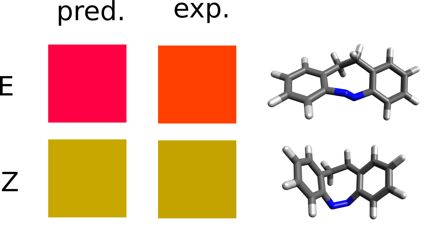
To make this rather abstract topic into something more concrete, we will try to simulate the experimental results obtained for an azobenzene derivative [Temps2009]:
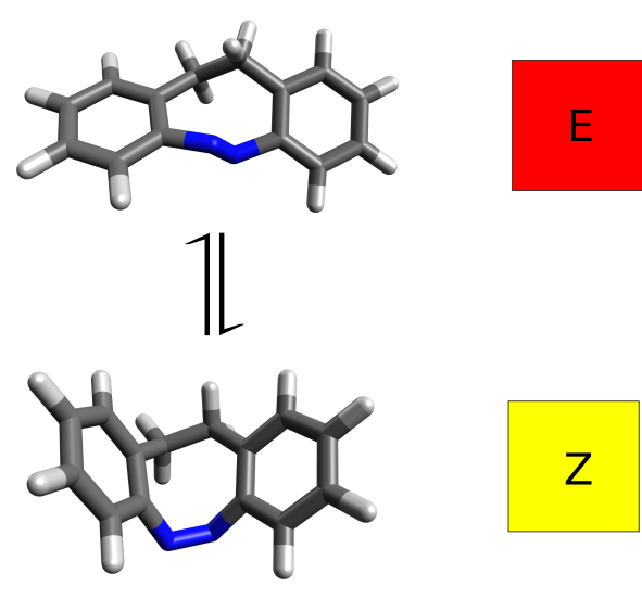
It turns out that the E and Z isomers have different colors - one is yellow and the other red - and the authors attribute this to a change in the lower energy band, assigned as a \(n-\pi^*\) transition. Let's see how we could have predicted these results from first principles.
TD-DFT
The time-dependent density functional theory (TD-DFT) is one of the most common approaches to predict UVVis spectra, because it is rather simple and not computationally too expensive. Its usage in ORCA is simple, for instance choosing the B3LYP functional and a triplet-zeta basis:
!B3LYP DEF2-TZVP CPCM(HEXANE)
%TDDFT
   NROOTS   30
END
* XYZfile 0 1 Eisomer_optimized.xyz
The %TDDFT automatically requests the excited-state calculation necessary for the prediction of the spectrum and the NROOTS flag controls the number of excited states you want to include.
Here we also used the CPCM as a solvation model for both the ground and the excited states to simulate the hexane used in the experiment, which for the excited state case means the LR-CPCM model by default. After the regular SCF, the TD-DFT header is printed:
------------------------------------------------------------------------------
                        ORCA TD-DFT/TDA CALCULATION
------------------------------------------------------------------------------

Input orbitals are from        ... AZOZ_TDDFT_HEX.gbw
CI-vector output               ... AZOZ_TDDFT_HEX.cis
Tamm-Dancoff approximation     ... operative
CIS-Integral strategy          ... AO-integrals
Integral handling              ... AO integral Direct
Max. core memory used          ... 4000 MB
Reference state                ... RHF
Generation of triplets         ... off
Follow IRoot                   ... off
Number of operators            ... 1
Orbital ranges used for CIS calculation:
 Operator 0:  Orbitals  16... 54  to  55...567
XAS localization array:
 Operator 0:  Orbitals  -1... -1
with details with respect to the orbital windows, memory used and integral algorithms.
Note
The default version of TD-DFT in ORCA makes use of the TDA approximation. This can be turned off by setting TDA FALSE under %TDDFT.
The necessary grids are build and the Davidson procedure starts:
------------------------
DAVIDSON-DIAGONALIZATION
------------------------

Dimension of the eigenvalue problem            ...  20007
Number of roots to be determined               ...     30
Maximum size of the expansion space            ...    300
Maximum number of iterations                   ...    100
Convergence tolerance for the residual         ...    1.000e-06
Convergence tolerance for the energies         ...    1.000e-06
Orthogonality tolerance                        ...    1.000e-14
Level Shift                                    ...    0.000e+00
Constructing the preconditioner                ... o.k.
Building the initial guess                     ... o.k.
Number of trial vectors determined             ...    300


                       ****Iteration    0****

   Memory handling for direct AO based CIS:
   Memory per vector needed      ...    14 MB
   Memory needed                 ...  1329 MB
   Memory available              ...  3000 MB
   Number of vectors per batch   ...   203
   Number of batches             ...     1
   Time for densities:            0.503
   Time for RI-J (Direct):        3.903
   Time for K (COSX):            45.512
   Time for XC-Integration:      21.118
   Time for LR-CPCM terms:        9.571
   Time for Sigma-Completion:     0.393
   Size of expansion space: 90
   Lowest Energy          :     0.092988177038
   Maximum Energy change  :     0.259251849588 (vector 29)
   Maximum residual norm  :     0.016689588426
   [...]
until convergence is reached according to the tolerances printed in the header.
Note that the RI and COSX approximations are also used to compute the necessary integrals for the TD-DFT solution. The error here is usually even smaller than in the SCF, and the calculation runs much faster (by a factor of about 10), so it is highly recommended to use these.
Printing of the excited states
Finally the converged states are printed:
------------------------------------
TD-DFT/TDA EXCITED STATES (SINGLETS)
------------------------------------

the weight of the individual excitations are printed if larger than 1.0e-02

STATE  1:  E=   0.089757 au      2.442 eV    19699.5 cm**-1 <S**2> =   0.000000
    50a ->  55a  :     0.039008 (c= -0.19750352)
    54a ->  55a  :     0.942532 (c=  0.97084090)

STATE  2:  E=   0.138303 au      3.763 eV    30354.1 cm**-1 <S**2> =   0.000000
    53a ->  55a  :     0.938086 (c=  0.96854831)
    54a ->  58a  :     0.027177 (c= -0.16485521)
[...]
It is important to have in mind that these energies actually are the vertical energy differences, or the energy of that state in the ground state geometry.
Below the energies, the contributions of each single excitation are printed, first with its relative contribution (these will be discussed later), followed by the eigenvector value.
The electronic spectrum
After a detailed printing of the CPCM correction, ORCA does the calculation of some necessary integrals:
-----------------------------
TD-DFT/TDA-EXCITATION SPECTRA
-----------------------------

Center of mass = ( -0.0082,  0.0205,  0.0077)
Calculating the Dipole integrals                  ... done
Transforming integrals                            ... done
Calculating the Linear Momentum integrals         ... done
Transforming integrals                            ... done
Calculating angular momentum integrals            ... done
Transforming integrals                            ... done
and the "spectrum" is printed:
-----------------------------------------------------------------------------
         ABSORPTION SPECTRUM VIA TRANSITION ELECTRIC DIPOLE MOMENTS
-----------------------------------------------------------------------------
State   Energy    Wavelength  fosc         T2        TX        TY        TZ
        (cm-1)      (nm)                 (au**2)    (au)      (au)      (au)
-----------------------------------------------------------------------------
   1   19699.5    507.6   0.047917124   0.80078   0.87904  -0.16736   0.00724
   2   30354.1    329.4   0.012327447   0.13370   0.05769   0.36102  -0.00597
   3   31373.4    318.7   0.023725133   0.24896  -0.48626   0.08573  -0.07183
   4   32906.2    303.9   0.002354014   0.02355  -0.04012  -0.14813   0.00027
   5   34099.1    293.3   0.176508288   1.70411   1.27793  -0.24569  -0.10310
[...]
The states and their respective vertical transition energies are printed again, now together with the oscillator strength and transition dipole moments. Strictly speaking, this is yet not a "spectrum" like the experimental one because we only have transition lines, not bands.
Plotting the calculated spectrum
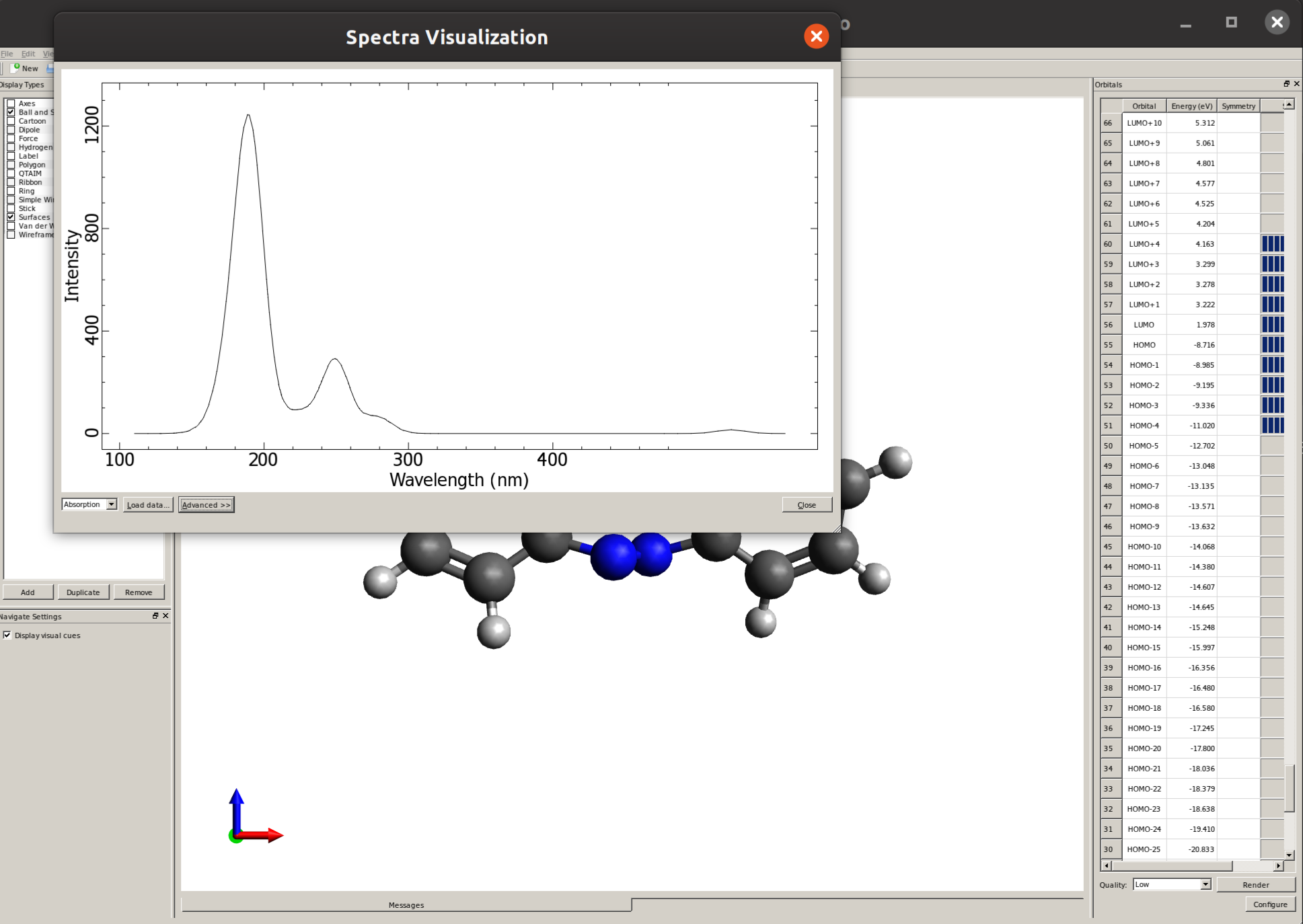
What we can do to approximate the experimental spectrum then is, e.g, convolute these lines with a Gaussian function to turn them into bands. This can be done easily by using Avogadro: open the output file, then go into "Extensions" and then "Spectra..." to open the "Spectra Visualization" window:
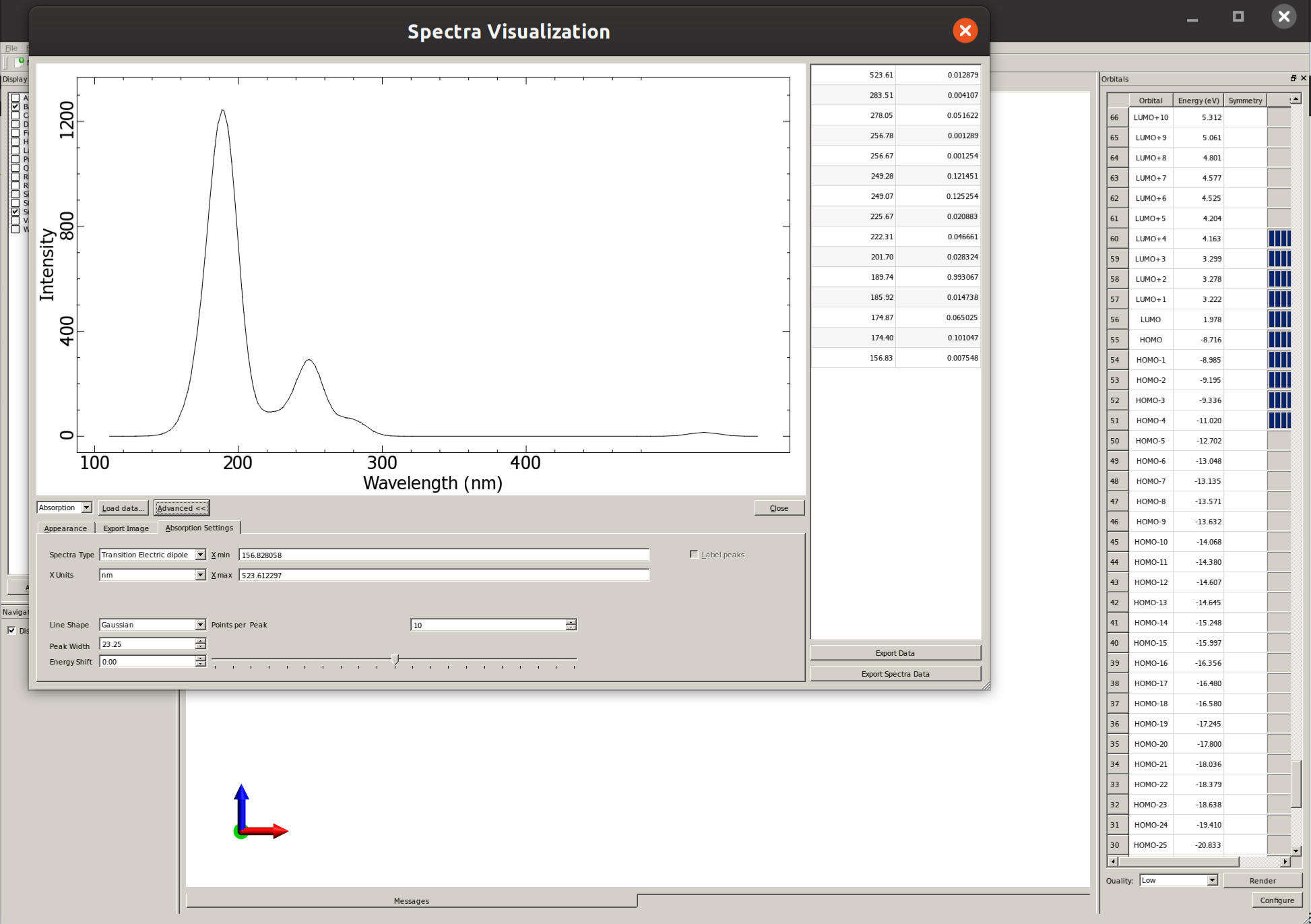
There you can click on "Advanced" and then "Absorption Settings" to set the details such as the line width and even "Export Spectra Data" to replot this graphic using a different software:
Back to the example
Here is a plot of the predicted spectrum for both the E and Z isomers obtained from the calculation above, using B3LYP and the DEF2-TZVP basis:
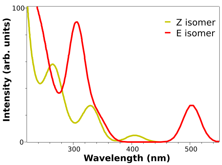
The two low energy peaks at about 507 and 417 nm for the E and Z isomers match quite well the experimental results of 490 and 404 nm. If one converts this wavelength to color and takes its complementary, the correspondence is fairly good:
Important
It is not that common that these results agree so well to the experiment, and here it can be somewhat accidental. It is much more prevalent that the predicted spectra is "shifted" by ±0.1 to ±0.5 eV and it is costumary in the literature to fix that, if there is any reference, to correct systematic errors.
Analysis of the excited states
The usual assignement for the spectral bands in azobenzenes is that the lower energy peak corresponds to the \(S_1\) state, that is of \(n-\pi^*\) character, while the higher \(S_2\) is a \(\pi-\pi^*\) state - which has major implications on the isomerization process.
We can make use of the calculated results to help with that complicated task, by checking on the composition of the excited states. As mentioned previously, it is printed in the TD-DFT output that the first excited state (of the E isomer) is composed of:
STATE  1:  E=   0.089757 au      2.442 eV    19699.5 cm**-1 <S**2> =   0.000000
    50a ->  55a  :     0.039008 (c= -0.19750352)
    54a ->  55a  :     0.942532 (c=  0.97084090)
Which means that the \(S_1\) state is composed of about 94% a HOMO to LUMO transition, from orbital 54 to orbital 55 (the "a" there means alpha orbital).
If you run a calculation using !LARGEPRINT on the main input, you can visualize these orbitals by opening the basename.out file directly in Avogadro, and they will be:
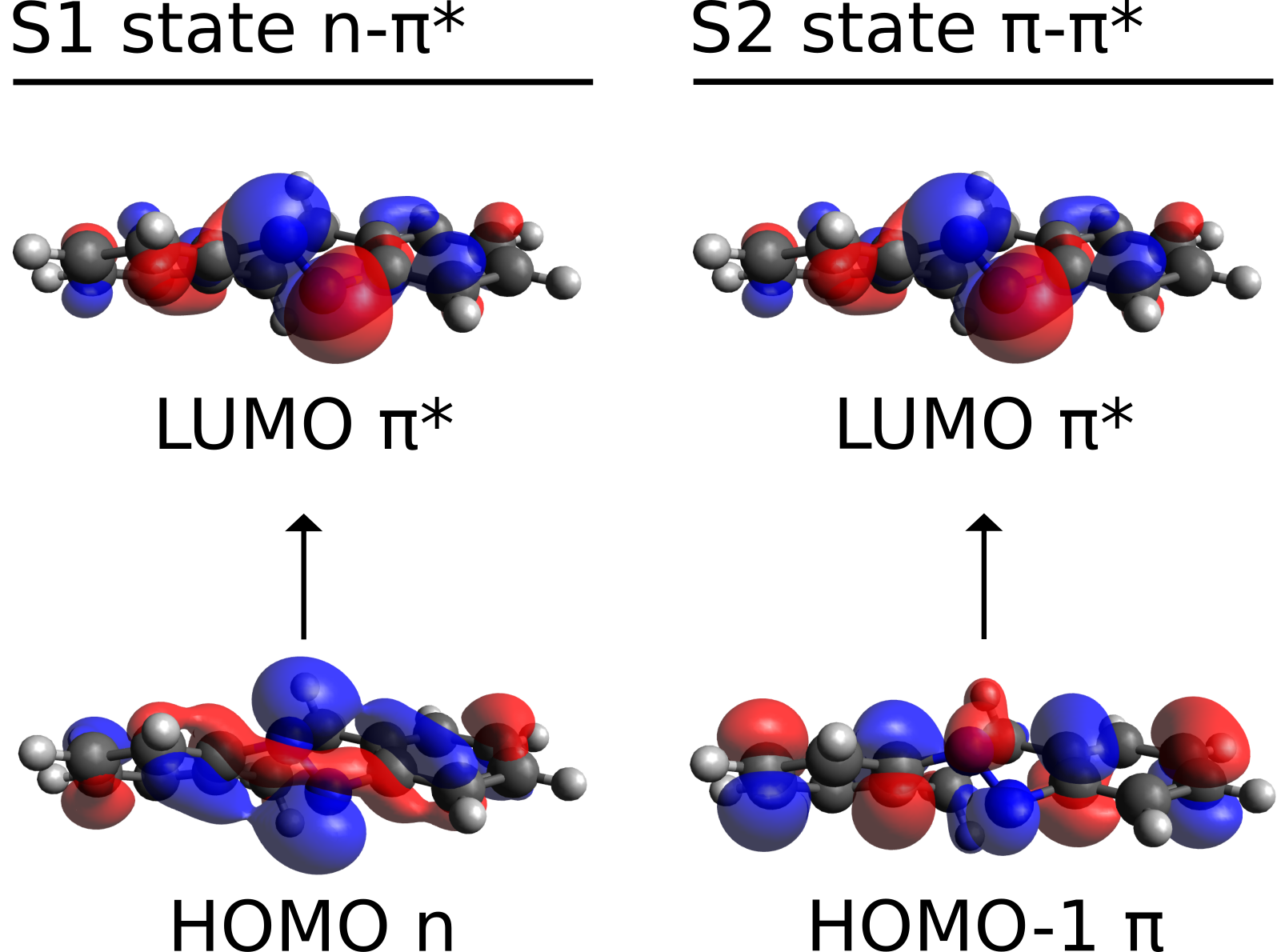
As you can see, the HOMO is a \(n\)-like molecular orbital, mostly located on the isolated electron pairs of the nitrogens, and the LUMO is a \(\pi^*\) orbital, primarily around the N=N bond, thus corroborating the suggested assignment.
We also printed the \(S_2\) main component, which is 94% HOMO-1 to LUMO transition. From the image above, it is also possible to see that the HOMO-1 now is more like a regular \(\pi\) orbital, and the \(\pi-\pi^*\) assignment seems like a good assumption. However, now we even have the information that it is from the ring orbitals to the N=N antibonding orbital.
Important
Avogadro counts orbitals starting from 1, but ORCA starts counting from 0. So orbital 54 in ORCA will be orbital 55 in Avogadro, and so on!
Natural transition orbitals (NTOs)
Another approach to investigate the nature of the excited states is to look at the NTOs of each transition [Martin2003]. These a more "compact" version of the molecular orbitals and can help interpreting more complex cases. Take, for instance, the excited state 13 of the E isomer:
STATE 13:  E=   0.213089 au      5.798 eV    46767.6 cm**-1 <S**2> =   0.000000
    51a ->  56a  :     0.502626 (c= -0.70896131)
    51a ->  57a  :     0.078981 (c= -0.28103567)
    51a ->  58a  :     0.067618 (c= -0.26003484)
    52a ->  56a  :     0.013149 (c=  0.11466855)
    52a ->  58a  :     0.032710 (c=  0.18085868)
    53a ->  57a  :     0.157493 (c= -0.39685415)
    53a ->  58a  :     0.102542 (c= -0.32022179)
There are at least seven large transitions involved, which might be quite confusing to untangle. Now, if one requests a TD-DFT calculation using DONTO TRUE:
!B3LYP DEF2-TZVP CPCM(HEXANE)
%TDDFT
   NROOTS   30
   DONTO    TRUE
END
* XYZfile 0 1 isomer_optimized.xyz
the excited states are also printed in terms of their NTOs:
------------------------------------------
NATURAL TRANSITION ORBITALS FOR STATE   13
------------------------------------------

Making the (pseudo)densities                       ... done
Solving eigenvalue problem for the occupied space  ... done
Solving eigenvalue problem for the virtual space   ... done
Natural Transition Orbitals were saved in AZOE_TDDFT_HEX.s13.nto
Threshold for printing occupation numbers 0.001000

E=   0.217964 au      5.931 eV    47837.6 cm**-1
   54a ->  55a  : n=  0.52307981
   53a ->  56a  : n=  0.45580888
   52a ->  57a  : n=  0.01323011
   51a ->  58a  : n=  0.00489879
   50a ->  59a  : n=  0.00203051
and the \(S_{13}\) is now described in terms of only two main transitions. These NTOs are saved in a file named basename.s13.nto, and can be printed using the orca_plot tool.
After generating the .cube files for orbitals 53-56, these can be plotted using Avogadro. Open the .cube file, go to "Extensions", then "Create Surfaces...", and on "Surface Type" select the MO. After clicking on "Calculate", the orbitals will show up:
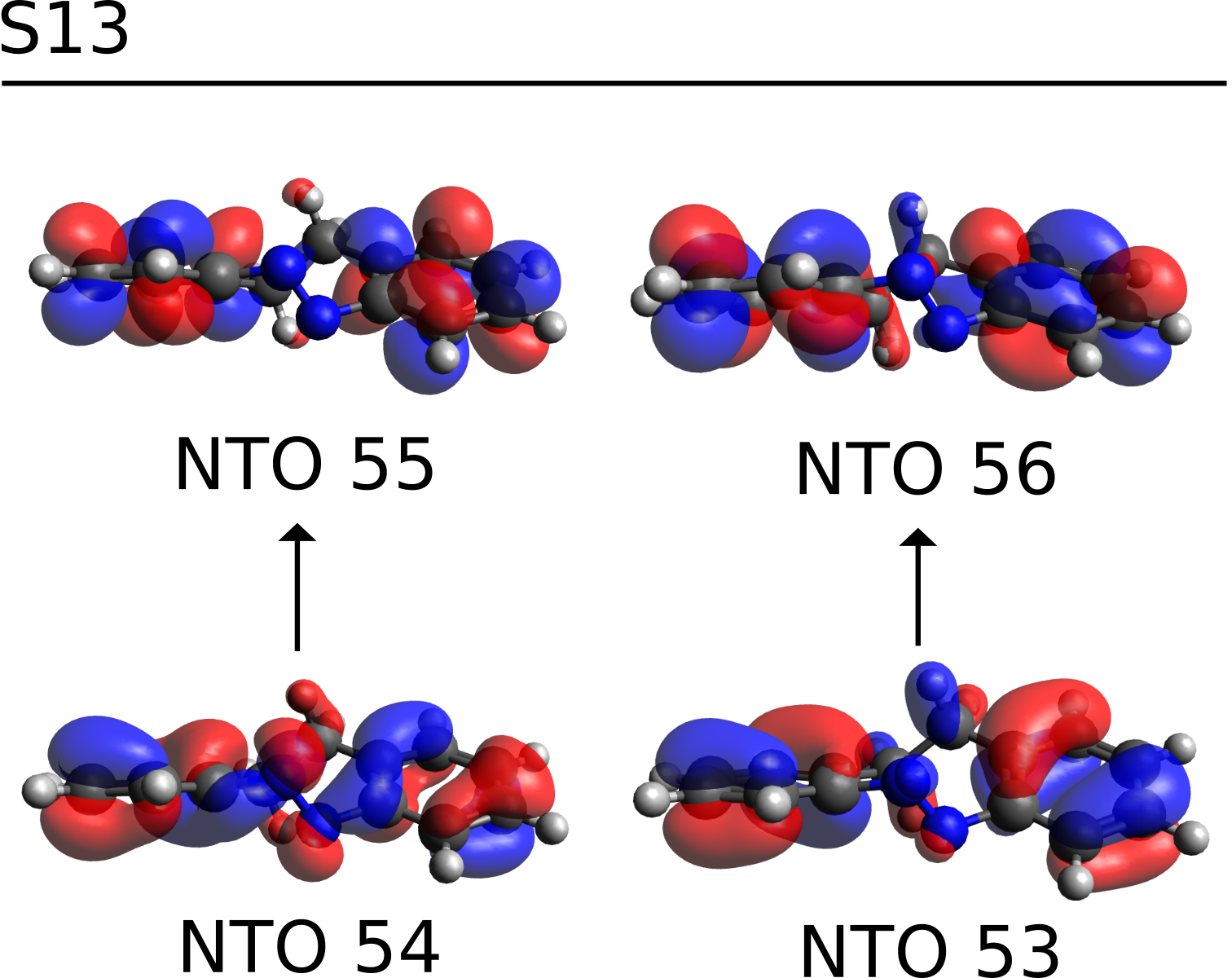
which are clearly \(\pi-\pi^*\) transitions on the aromatic rings, and \(S_{13}\) can then be assigned as such.
A higher level method - STEOM-DLPNO-CCSD
As shown above, TD-DFT can be successful in many cases when trying to predict excited states, however one can not know a priori if a given functional will work or not and different functionals are bound to give different results.
In order to avoid this trial-and-error between functionals, an ab initio unparametrized method is sometimes a better choice. In ORCA, many of these methods are available, but for the sake of simplicity we will show here one that has a very good accuracy, still at an affordable computational cost: the Similarity Transformed Equation of Motion CCSD (STEOM-CCSD).
The STEOM-CCSD is a method that also includes Correlation energy into the calculation of the excited states, thus increasing the quality of the prediction [Iszak2019a]. It is in itself a heavy method and very computational demanding, but the ORCA team has recently developed The DLPNO scheme version of it (DLPNO-STEOM), that presents a much better scaling and it is not much costlier than TD-DFT [Iszak2019b].
In order to use that, just optimize your geometry somehow and run:
!STEOM-DLPNO-CCSD DEF2-TZVP DEF2-TZVP/C RIJCOSX CPCM(HEXANE)
%MDCI
   NROOTS  15
   DOSOLV  TRUE
END
* XYZFILE 0 1 AZOE_HEX.xyz
As in other DLPNO or correlated methods using the RI, the /C basis is necessary for the calculation. We also added the CPCM correction for both the ground and excited states, here the latter is invoked by setting DOSOLV TRUE under %MDCI, which is the block that controls these calcualtions.
The MAXITER 100 defines the maximum number of iterations during the many steps of STEOM, and sometimes it is necessary to increase it to achieve convergence.
Note
As with the other CC methods, a large amount of memory might be needed. Also, be sure you use a sufficiently large basis, of at least the size of DEF2-TZVPP for consistent results.
The output printed is much larger than that of TD-DFT, for there are many more steps necessary to conclude the overall computation. In summary what is done is:
First a regular DLPNO-CCSD calculation is performed.
That is followed by a simple CIS calcuation, that is necessary to reduce the active space.
Then both a DLPNO-IP-EOM and a DLPNO-EA-EOM are made.
Several integrals are transformed.
Finally, the STEOM-CCSD step starts:
---------------------------------------------------
           RHF STEOM-CCSD CALCULATION
---------------------------------------------------

EOM type                                   ... STEOM
Multiplicity                               ... singlet
Solver                                     ... Davidson
Convergence check                          ... for each root separately
Convergence threshold                      ... 1.00E-05
Root homing                                ... on
Preconditioning update                     ... CIS
Reduced space size (times number of roots) ... 40
Number of roots in the CIS initial guess   ... 600
Number of roots to be optimized            ... 15
Number of amplitudes to be optimized       ... 20007
[...]
The equations are solved rootwise by default, and after everything converges, the results are printed:
------------------
STEOM-CCSD RESULTS
------------------

IROOT=  1:  0.090940 au     2.475 eV   19959.0 cm**-1
  Amplitude    Excitation
   0.674029    50 ->  55
   0.249536    50 ->  59
   0.127342    50 ->  61
   0.120800    52 ->  55
  -0.595419    54 ->  55
  -0.194231    54 ->  59
  Ground state amplitude: -0.005413
  [...]
Similarly to TD-DFT, the square of the amplitudes is the percentage of that excitation in the final state. The solvent shift is done, some other integrals are calculated and the "spectrum" is printed:
-----------------------------------------------------------------------------
         ABSORPTION SPECTRUM VIA TRANSITION ELECTRIC DIPOLE MOMENTS
-----------------------------------------------------------------------------
State   Energy  Wavelength   fosc         T2         TX        TY        TZ
        (cm-1)    (nm)                  (au**2)     (au)      (au)      (au)
-----------------------------------------------------------------------------
   1   19779.9    505.6   0.014001484   0.23304   0.47586   0.07963   0.01518
   2   34947.2    286.1   0.003239579   0.03052   0.02193   0.17096   0.00422
   3   35835.7    279.1   0.032206604   0.29587   0.53403   0.10234   0.01138
   4   38594.7    259.1   0.002685224   0.02290   0.06150   0.13658   0.00042
   5   40165.6    249.0   0.217313109   1.78118   1.30981   0.25574   0.01007
   6   44084.8    226.8   0.039175298   0.29255   0.40132   0.15728   0.26059
The output file can be opened in Avogadro and the spectrum plotted as explained above in Plotting the calculated spectrum:
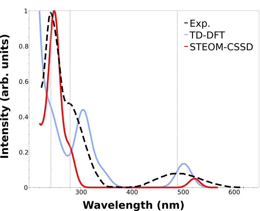
Here we added the gray vertical lines to guide the eye to the first three peaks of the spectrum. As you can see, although TD-DFT works well to predict the first, the higher energy ones are largely displaced.
That can happen when these states are significantly different, and the associated error is not comparable. One advantages of the STEOM is that there is a more balanced treatment of different excited states and such situations and avoided.
The calculated results are now well in line with the experiment through the whole spectrum, except for a small deviation on the intensities. We can arrange these results in a table to facilitate visualization: below there is comparison of the energy error of the first three peaks measured for the E isomer. The TD-DFT can be as high as 1 eV!
Peak |
TD-DFT |
STEOM |
Exp. |
|---|---|---|---|
1 |
4.23 |
5.06 |
5.14 |
2 |
3.83 |
4.42 |
4.43 |
3 |
2.46 |
2.45 |
2.53 |
Important
Even if the predicted spectrum matches the experiment, the calculation is still not reproducing exactly what happens during light absorption. The full experimental spectra must also include vibrational resolution, and maybe even vibronic coupling. That can be included with the ORCA_ESD module.