NMR spectra
ORCA can also be used to predict NMR spectra, both in the form of NMR shifts for any nucleus and J couplings for any pair of nuclei. Here we will discuss both cases, exemplifying with an organic acid and toluene.
C-NMR spectra of the propionic acid
Lets first compute the C-NMR shifts for the propionic acid in chloroform, for which the experimental data can be found in the SDBS database:
A guess geometry should be first optimized (see Geometry optimization), for intance, with:
!B3LYP DEF2-TZVPP D3 OPT
* xyzFile 0 1 guess_propionic.xyz
Important
Always have in mind that NMR shifts are quite dependent on the conformer you choose. A conformer search or even a Boltzmann weighting might be necessary!
Having your structure optimized, the NMR shieldings are requested by adding NMR on the first input line and adding the specifics under the %EPRNMR block, that should always come after the geometry section. To request the NMR shieldings, just add {SHIFT} after the atom assignments:
!B3LYP DEF2-TZVPP NMR
* xyzFile 0 1 propionic_optimized.xyz
%EPRNMR
     NUCLEI = ALL C {SHIFT}
END
Note
The default algorithm uses Gauge-Independent Atomic Orbitals (GIAOs, [Ditchfield1973] and [Pulay1990]). This is quite important in NMR calculations and we do not recommended turning this off unless you really know what you are doing.
If one just types NMR on the first line, without specifying the nuclei below, then shieldings for all the atoms will calculated. Specific atoms can be added as a list, following what is described in Predicting EPR.
After a successful SCF calculation, the output starts with the heading:
------------------------------------------------------------------------------
                              ORCA EPR/NMR CALCULATION
------------------------------------------------------------------------------

GBWName                      ... prop.gbw
Electron density file        ... prop.scfp
Spin density file            ... prop.scfr
Treatment of gauge           ... GIAO (approximations 1/2el = 0,0)
Details of the CP(SCF) procedure:
       Solver   = POPLE
       MaxIter  =    64
       Tolerance=    1.000e-03
       COSX Grid=     1
       Op-0     =   0- 19 =>  20-238
Multiplicity                 ... 1
g-tensor                     ... 0
NMR chemical shifts          ... 1
NMR spin-spin couplings      ... 0
NMR spectrum                 ... 0
Number of nuclei for epr/nmr ... 3
Now, you can see some details of the calculation, with the GIAO as the Treatment of gauge, and the number of nuclei that will be covered. Then the GIAO integrals are solved:
One-electron GIAO integrals (SHARK)     ... done
Calculating G(B)[P]                     ... (RI-J: SHARK-ok) (COSX-ok) (add-J+K:ok) => dG/dB done
DFT XC-terms                            ... done
Extracting occupied and virtual blocks  ...
Operator  0  NO=  20 NV= 219
Transforming and RHS contribution       ... done
Adding eps_i * S(B)_ai terms            ... done
Projecting overlap derivatives          ... done
Building G[dS/dB_ij] (COSX)             ... done
Transforming to MO basis                ... done
Summing G[dS/dB_ij] into RHS contribs.  ... done

GIAO profiling information:
  Total GIAO time               ...       3.1 sec
     GIAO 1-electron integrals  ...       0.0 sec (  0.5%)
     GIAO G(dS/dB) terms        ...       0.3 sec (  8.9%)
     GIAO RI-J                  ...       0.3 sec (  9.2%)
     GIAO COSX                  ...       0.9 sec ( 30.5%)
     GIAO XC-terms              ...       1.3 sec ( 43.1%)
     Right hand side assembly   ...       0.0 sec (  0.3%)

GIAO right hand side done
followed by the CP-SCF calculations necessary to derivatives and finally the chemical shieldings are computed:
---------------
CHEMICAL SHIFTS
---------------

Note: using conversion factor for au to ppm alpha^2/2 =   26.625677252
GIAO: Analytic para- and diamagnetic shielding integrals (SHARK)       ...done
 --------------
 Nucleus   0C :
 --------------

Diamagnetic contribution to the shielding tensor (ppm) :
           252.962          6.663        -0.018
             5.897        239.026        -0.015
            -0.013         -0.008       234.344

Paramagnetic contribution to the shielding tensor (ppm):
           -71.688         -3.304         0.010
            -1.624        -65.200         0.001
            -0.015         -0.006       -67.811

Total shielding tensor (ppm):
           181.275          3.359        -0.008
             4.273        173.826        -0.014
            -0.027         -0.014       166.532


 Diagonalized sT*s matrix:

 sDSO           234.344          236.632          255.357  iso=     242.111
 sPSO           -67.811          -64.414          -72.474  iso=     -68.233
        ---------------  ---------------  ---------------
 Total          166.532          172.218          182.882  iso=     173.878
First, you can see that the results for carbon number 0 are printed (0C), with all its specific contributions, and the other atoms requested follow in order. Usually, the number that we actually measure is related to the isotropic shift, that is printed after iso=.
Note
Chemically equivalent nuclei might have slight different shieldings, due to geometric asymmetries. In that case, the best thing to do is just average them.
At the end of the file, a summary is printed, with the isotropic part and the anisotropy:
--------------------------------
CHEMICAL SHIELDING SUMMARY (ppm)
--------------------------------

  Nucleus  Element    Isotropic     Anisotropy
  -------  -------  ------------   ------------
      0       C          173.878         13.507
      1       C          154.867         35.163
      5       C            2.913       -144.729
Important
These NMR shieldings are not comparable the experimental ones! One still needs to compute a reference shielding or use an internal standard to convert to proper experimental shifts. Please read the next sections on how to do that.
Calculating the reference NMR shieldings
Similarly to the experiment, the absolute values of the shieldings have no much meaning without a reference value, and we might need to compute those as well. In the case of 13C-NMR and 1H-NMR, you can use TMS (Tetramethylsilane), which is also the usual experimental reference for that. Just optimize and compute the C-NMR of TMS by running the input such as:
!B3LYP DEF2-TZVPP NMR
* xyzFile 0 1 TMS_optimized.xyz
%EPRNMR
     NUCLEI = ALL C {SHIFT}
END
and you will get:
--------------------------------
CHEMICAL SHIELDING SUMMARY (ppm)
--------------------------------

  Nucleus  Element    Isotropic     Anisotropy
  -------  -------  ------------   ------------
      1       C          183.069          9.263
      2       C          183.082          9.249
      3       C          183.076          9.255
      4       C          183.077          9.255
Now, the average value of the C-NMR shieldings can be used to compute the shifts that are comparable to the experimental by using:
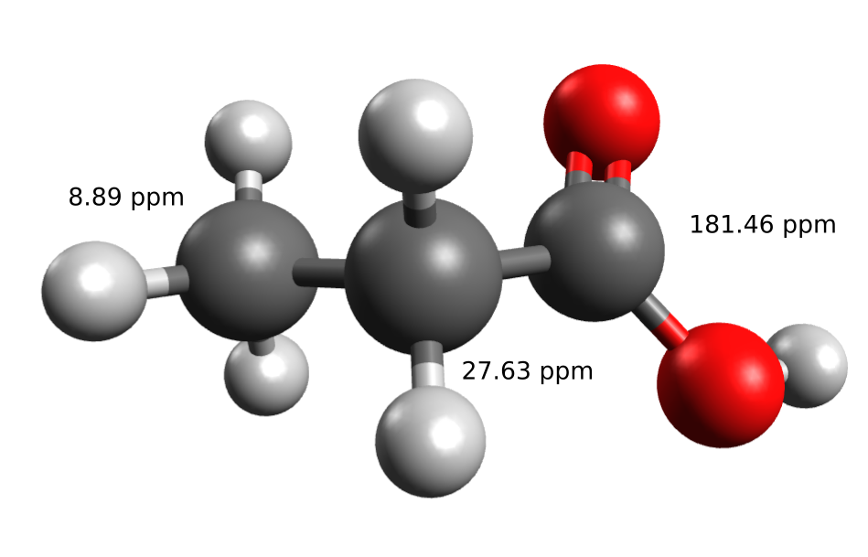
and the results for three different calculation levels, using the B3LYP-optimized structures, are:
Method |
\(\delta_1\) |
\(\delta_2\) |
\(\delta_3\) |
|---|---|---|---|
HF-RIJCOSX |
10.5 |
27.1 |
184.1 |
BP |
9.8 |
29.0 |
176.8 |
B3LYP |
9.2 |
28.2 |
180.2 |
Exp. |
8.9 |
27.6 |
181.5 |
Note
Have in mind that the refence should always use the same level of theory as the target molecule, including any solvation effects or approximations such as the RI.
The use of an internal standard
Instead of calculating a reference molecule, you can also just apply a constant shift to the calculated peaks, so that one of them is equal to a know value.
One could use the value of an assigned methyl or an aromatic H or C and benefit from possible error cancellations. This also makes more sense if the reference is too different from the target molecule or it is somehow complicated to simulate, like phosphoric acid for 31P-NMR.
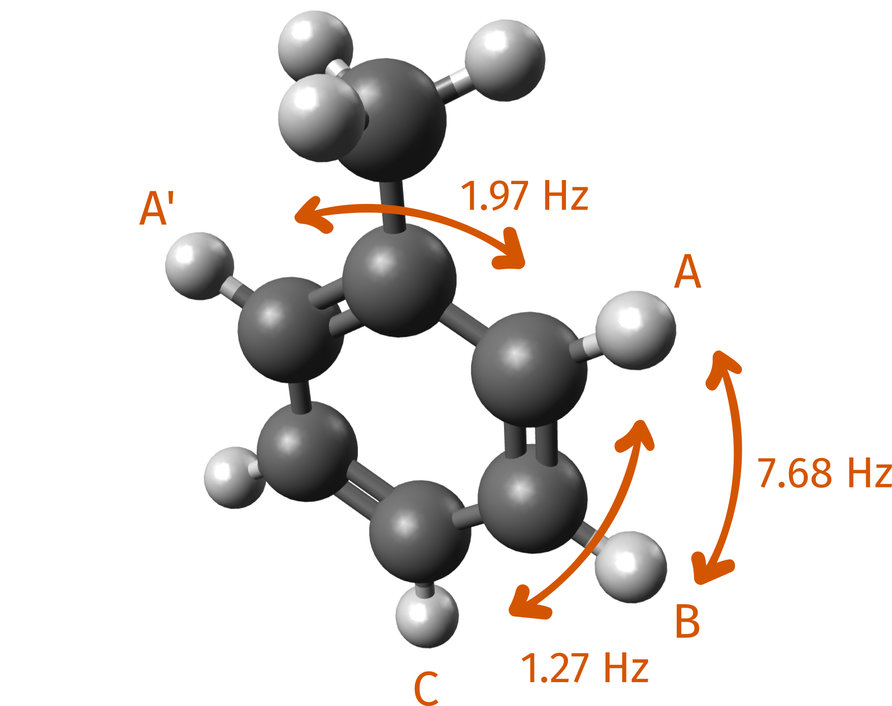
H-NMR of toluene and J couplings
The same scheme can be used to predict the H-NMR and the couplings. Let's do it for toluene, for which the reference values can also be found at SDBS. Here we highlight some of the J couplings between hydrogen atoms, as labeled on the database:
Again, first we optimize the structure and then compute the shieldings. This time, we will use one of the Implicit Solvation Models to include the effect of chloroform:
!B3LYP PCSSEG-2 AUTOAUX NMR CPCM(CHLOROFORM)
* xyzFILE 0 1 TOL_optimized.xyz
%EPRNMR
     NUCLEI = ALL H {SHIFT, SSALL}
END
Here we used the pcSseg-2 basis, which is well suited for NMR calculations, and the AUTOAUX flag was chosen to automatically build the necessary auxiliary basis.
After the output that was already discussed, the coupling section is printed:
                 NMR SPIN-SPIN COUPLING CONSTANTS
                 ================================

Number of nuclear pairs to calculate something:       22
                                                    ----
Number of nuclear pairs to calculate DSO   terms:     22
Number of nuclear pairs to calculate PSO   terms:     22
Number of nuclear pairs to calculate FC    terms:     22
Number of nuclear pairs to calculate SD    terms:     22
Number of nuclear pairs to calculate SD/FC terms:     22
                                                    ----
Number of nuclei to calculate PSO   perturbations:     6
Number of nuclei to calculate SD/FC perturbations:     6
Since we used the SSALL option, all components of the coupling are included. For the specifics on how to turn these on and off, please check the ORCA manual (must log in).
Then comes a detailed description of these couplings, starting from one atom and listing closest neighbors (there is a cutoff radius of \(5\) Å):
================================
Nucleus = H    0 interacts with:
H 3, H 7, H 9, H 11, H 12
================================
and all couplings are listed, in Hz, as:
-----------------------------------------------------------
 NUCLEUS A = H    0 NUCLEUS B = H    3
 (  1H  gnA =  5.586   1H  gnB =  5.586) r(AB) =     2.4640
-----------------------------------------------------------
[...]
Diagonalized sT*s matrix:

ssDSO           -3.702           -1.293            3.910  iso=      -0.362
ssPSO            2.632            0.729           -2.823  iso=       0.179
ssFC             6.797            6.797            6.797  iso=       6.797
ssSD             0.117           -0.084            0.176  iso=       0.069
ssSD/FC          0.056            0.207           -0.269  iso=      -0.002
---------------  ---------------  ---------------  ----------------
Total            5.900            6.356            7.791  iso=       6.682
Once more, the value that correspond to what most experiment measures comes after the iso=.
Important
The values are printed in Hz, so in order to convert them to ppm one has to take into account the equipment's frequency. In our case, the database says it was measured in 300 MHz NMR, so that the coupling in ppm would be:
A summary of the results is given below:
Coupling |
Calculated (ppm, Hz) |
Experiment (ppm, Hz) |
|---|---|---|
A - A' |
0.006, 1.88 |
0.007, 1.97 |
A - B |
0.022, 6.68 |
0.026, 7.68 |
A - C |
0.004, 1.16 |
0.004, 1.27 |
NMR prediction using double-hybrids
In ORCA, the NMR properties can also be computed using the double-hybrid functionals, that profit from adding MP2 correlation to DFT [Neese2018]. These can be used by setting the NOFROZENCORE flag, together with the desired functional:
!RI-B2PLYP PCSSEG-3 AUTOAUX NMR
In that case the NMR calculation runs twice. First, ORCA does only the DFT part:
*****************************************
*        EPRNMR WITH SCF DENSITY        *
*****************************************
and, at the end, the analytic MP2 derivatives are computed:
Calculating analytic MP2 second derivatives ... (>DSD-TOL_H.last_mp2_re) done
That can take some time, while no other message will be printed. After finishing these derivatives, the MP2 part is added and the results are printed under the header:
**************************************
*  EPRNMR WITH MP2 RELAXED DENSITY   *
**************************************
In our experience, there provide the most reliable results at a cheaper level of theory and can be used even together with spin-scaled double-hybrids such as the RI-DSD-PBEP86.
Tips
The pcSseg-2 is recommended for HF/DFT and pcSseg-3 for MP2/double-hybrids.
TPSS, TPSSh or DSD-PBEP86 D3BJ are in general the best methods.
Starting structures
1-propionic acid
C         -2.02927       -0.06431        0.00093
C         -0.75947        0.77416       -0.00117
H         -2.05906       -0.70449       -0.87666
H         -2.90593        0.57776       -0.00053
H         -2.05900       -0.70031        0.88157
C          0.48217       -0.08028       -0.00022
H         -0.71468        1.42253        0.87662
H         -0.71544        1.41914       -0.88152
O          1.59402        0.67317        0.00068
H          2.38322        0.10903        0.00141
O          0.52000       -1.27957       -0.00039
TMS
Si         0.00000        0.00000        0.00000
C          0.00000        0.00000        1.89465
C          1.78629        0.00000       -0.63155
C         -0.89314       -1.54697       -0.63155
C         -0.89314        1.54697       -0.63155
H         -1.02044        0.00000        2.29370
H          0.51022        0.88372        2.29370
H          0.51022       -0.88372        2.29370
H          1.82238        0.00000       -1.72665
H          2.33260        0.88372       -0.28352
H          2.33260       -0.88372       -0.28352
H         -0.91119       -1.57822       -1.72665
H         -1.93163       -1.57822       -0.28352
H         -0.40097       -2.46195       -0.28352
H         -0.91119        1.57822       -1.72665
H         -1.93163        1.57822       -0.28352
H         -0.40097        2.46195       -0.28352
Toluene
H         -1.36375       -2.14710       -0.00000
C         -0.81841       -1.20707       -0.00000
C          0.57773       -1.21178        0.00000
H          1.10440       -2.16317        0.00000
C          1.29013       -0.00662        0.00000
C          2.78990        0.00393        0.00000
C          0.58296        1.20255        0.00000
H          1.11797        2.14948        0.00000
C         -0.81284        1.20580       -0.00000
H         -1.35324        2.14861       -0.00000
C         -1.51325        0.00108       -0.00000
H         -2.59986        0.00360       -0.00000
H          3.19906       -1.01171       -0.00000
H          3.16332        0.51620        0.89251
H          3.16332        0.51620       -0.89251