Calculating accurate energy barriers
Besides studying the mechanistic details of chemical reactions, ORCA can also be used to calculate accurate energy barriers, and thus predict reaction rates to a certain accuracy.
It must be clear here that it is rather difficult to compare the absolute values of the experimental energy barriers with the calculates ones. First, because these "experimental" values are never measured directly, but obtained from measured data only after a series of assumptions.
Second because, unless your are modeling the solvent explicitly, there will always be a relatively large error associated to solvation. And that is to say the least if one also does not account for conformational entropy, transmission coefficients and so on.
Study case: the Diels-Alder reaction
Still, it does make sense to compare relative reaction energy barriers and rates, and we will show here how one could do that for a classic Diels-Alder (DA) reaction between cyclopentadiene and some dieneophiles:
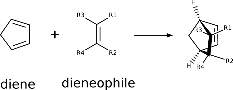
That is an important reaction, that conserves all of the atoms from the reactants, and particularly useful to synthesize chiral compounds. Its reaction rate varies drastically with the nature of the reactants, from \(10^{-8}\) to \(10^{2} s^{-1}\) [Guo2012], and its known that electron-withdrawing groups on the dieneophile accelerate the formation of the cyclic products:
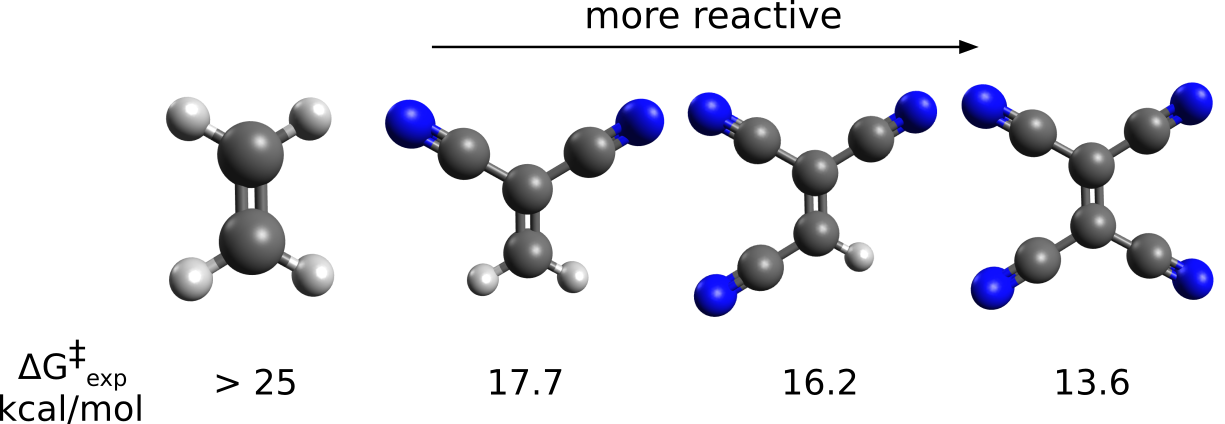
Let's try to investigate the relative barrier heights for the reaction between cyclopentadiene and the cyanide compounds above using the NEB-TS method to find the transition states, and investigate the effect of adding proper Correlation energy to it.
First, the transition state
The transition state (TS) for DA reactions is nothing unusual, except for the fact that three double bonds are being broken and two single bonds are being formed at the same time, which is sometimes hard to track using the usual TS-search algorithms that rely on a single coordinate search.
By using ORCA's NEB-TS method, the TS search is made much simpler, and all that is needed are the structures of the reactant and products. To optimize these using, e.g, B3LYP and a good DEF2-TZVP basis, one can use:
!B3LYP D4 DEF2-SVP OPT FREQ CPCM(TOLUENE)
* XYZFILE 0 1 4CN_reactant.xyz
Here we are using the D4 correction [Grimme2017] to account for dispersion interaction, which is key in this case, and the CPCM solvation model [Truhlar2009] to include solvation effects to some extent.
After checking that both reactant and product are real minima, without any negative frequencies, one can already start the NEB-TS calculation using the optimized structures:
!B3LYP D4 DEF2-SVP NEB-TS FREQ CPCM(TOLUENE)
%NEB
      NEB_END_XYZFILE "4CN_product_optimized.xyz"
END
* XYZFILE 0 1 4CN_reactant_optimized.xyz
The new keywords here are the NEB-TS and FREQ on the main input, and the name of the file containing the product geometry under %NEB. If everything goes well, a TS having a single negative frequency of about \(-368cm^{-1}\) will be automatically found:
Calculating the energy barrier
With the TS and reactant in hands, one can immediately compute the \(\Delta G^{\ddagger} = G^o_{TS} - G^o_{reactant}\) from the Gibbs free energy difference between them. Here is a table summarizing the results for the three cyanides shown above:
Compound |
B3LYP |
Exp. |
|---|---|---|
2 CN |
9.90 |
17.7 |
3 CN |
10.69 |
16.2 |
4C |
10.21 |
13.6 |
Well, that is actually not very helpful, since there is not even a clear trend! There is no clear trend resulting from the B3LYP calculation, however, the geometries look fine and the transition states are indeed saddle-points on the potential energy surface. Can we get something better than this?
Using DLPNO-CCSD(T) to correct the electronic energy
In general DFT is known to reproduce geometries and frequencies with reasonable quality for its low cost, but the energies are definitely a weak point. And they are even worse if the system studied is outside the training set of the functionals, which normally do not included transition states or atypical bonding situations.
There is where higher level ab initio methods should be used to compute the electronic energy of these systems. Correlated methods such as CCSD(T) are unparametrized, based on real physical principles and should truly reproduce the experimental results.
Using those methods together with the The DLPNO scheme developed by the ORCA team allows for fast a accurate calculations of these barriers task. To compute an accurate electronic energy in this case, we could take the DFT geometry and run:
!DLPNO-CCSD(T) DEF2-TZVPP DEF2-TZVPP/C
* XYZFILE 0 1 4CN_reactant_optimized.xyz
for both the reactant and the TS.
Converting \(E_{el}\) to \(G^o\)
In order to transform the DLPNO-CCSD(T) electronic energy (\(E_{el}\)) into a true \(G^o\), we have to include the vibrational corrections already discussed in the Thermodynamics section. As DFT predicts frequencies relatively well, we can use the correction obtained previously here.
To account for solvation, we can also take the \(\Delta G_{solv}\) presented in the Implicit Solvation Models section, as computed with DFT and add them up to obtained a better final \(\Delta G^{\ddagger}\):
Using these results, our updated table is now:
Compound |
B3LYP |
CCSD(T) |
Exp. |
|---|---|---|---|
2 CN |
9.90 |
14.71 |
17.7 |
3 CN |
10.69 |
12.73 |
16.2 |
4 CN |
10.31 |
9.48 |
13.6 |
And the patter is clearly there. We can even plot a graphic to show that there is indeed a linear correlation between the calculated and the experimental energy barriers:
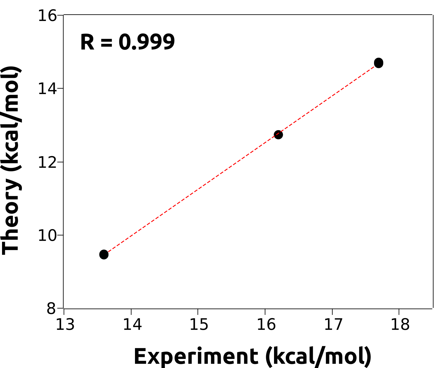
That means now we could, in principle, use this model to predict the experimental reaction barriers for unknown compounds with quite good accuracy, by calculating them and adjusting them to the fit!
Important
Again: it is very unlikely that the predicted and measured energy barriers will be equal, unless by coincidence. We not necessarily calculating the same quantity that was measured, but there should be relations like the one demonstrated above.
Starting structures
Reactant 2 CN
C         -3.69069       -0.24255       -3.05179
C         -3.57337       -0.78190       -1.82588
C         -4.57294       -0.54798       -0.84072
N         -5.39811       -0.33921       -0.05153
C         -2.43977       -1.57564       -1.49371
N         -1.51125       -2.22351       -1.23872
C         -2.11514        2.97164       -2.46395
C         -2.75801        2.94686       -1.10748
C         -1.82097        2.05962       -0.34096
H         -3.76291        2.51806       -1.15405
H         -2.80319        3.94828       -0.67099
C         -0.81416        1.66412       -1.13627
C         -0.99670        2.22898       -2.45201
H         -2.92766       -0.38759       -3.81222
H         -4.53742        0.38354       -3.32077
H         -1.94095        1.79488        0.69929
H         -2.49714        3.51913       -3.31237
H         -0.32049        2.07163       -3.27893
H          0.01334        1.02833       -0.85638
Product 2 CN
C         -3.20025        0.72134       -2.78548
C         -3.00842        0.13368       -1.34492
C         -4.31274       -0.11620       -0.70067
N         -5.34079       -0.28100       -0.18784
C         -2.20903       -1.10215       -1.36536
N         -1.58073       -2.07860       -1.39072
C         -2.57948        2.13393       -2.67804
C         -2.95544        2.53312       -1.25252
C         -2.28011        1.30743       -0.61598
H         -4.03779        2.57885       -1.09093
H         -2.51589        3.48780       -0.93519
C         -0.88730        1.50339       -1.17636
C         -1.08955        1.99428       -2.51692
H         -2.70739        0.12618       -3.56413
H         -4.26210        0.80563       -3.04971
H         -2.31744        1.29698        0.47604
H         -2.88251        2.84043       -3.45175
H         -0.33630        2.05640       -3.28724
H          0.03572        1.09522       -0.79171
Reactant 3 CN
C         -3.69898       -0.23681       -3.01835
C         -3.57195       -0.75519       -1.78419
C         -4.80664        0.54628       -3.43654
C         -4.55433       -0.56516       -0.77237
N         -5.70215        1.19542       -3.78131
N         -5.35261       -0.39983        0.05254
C         -2.39886       -1.49200       -1.46183
N         -1.42999       -2.08557       -1.22834
C         -2.16113        2.90081       -2.48911
C         -2.79788        2.88278       -1.12904
C         -1.84985        2.00691       -0.36196
H         -3.80037        2.44838       -1.16469
H         -2.84751        3.88655       -0.69946
C         -0.83661        1.62434       -1.15570
C         -1.03013        2.17737       -2.47476
H         -2.91467       -0.37452       -3.75726
H         -1.96469        1.74575        0.68017
H         -2.55493        3.43897       -3.33913
H         -0.34955        2.03081       -3.30051
H          0.00267        1.00519       -0.87184
Product 3 CN
C         -3.21165        0.73346       -2.79907
C         -3.05715        0.14686       -1.35153
C         -4.59355        0.81756       -3.28802
C         -4.33041       -0.09422       -0.64696
N         -5.67828        0.90014       -3.68685
N         -5.32012       -0.26103       -0.06541
C         -2.26700       -1.09612       -1.38224
N         -1.63017       -2.06502       -1.43179
C         -2.59535        2.15521       -2.66873
C         -2.94766        2.54448       -1.23191
C         -2.28872        1.30023       -0.62078
H         -4.02563        2.61090       -1.05062
H         -2.48524        3.48659       -0.90886
C         -0.89880        1.47289       -1.19641
C         -1.10174        2.00115       -2.52318
H         -2.63399        0.15306       -3.53289
H         -2.30987        1.27987        0.47185
H         -2.89272        2.88862       -3.42118
H         -0.36528        1.99552       -3.31368
H          0.01318        1.01032       -0.84542
Reactant 4 CN
C         -3.76429       -0.37684       -3.05298
C         -3.60332       -0.85967       -1.80350
C         -4.84674        0.48726       -3.38148
C         -2.83647       -0.67438       -4.09120
C         -4.50871       -0.52662       -0.75671
N         -5.72595        1.19981       -3.63289
N         -2.07298       -0.91406       -4.92930
N         -5.24903       -0.23911        0.08783
C         -2.49977       -1.69300       -1.46447
N         -1.59559       -2.36605       -1.19547
C         -2.03189        2.63992       -2.56556
C         -2.72195        2.85001       -1.24813
C         -1.92245        1.95807       -0.34275
H         -3.76788        2.53469       -1.29212
H         -2.66422        3.89444       -0.93118
C         -0.93044        1.37401       -1.03374
C         -0.99859        1.79618       -2.41214
H         -2.10952        1.83559        0.71465
H         -0.18080        0.70157       -0.64011
H         -0.30576        1.47983       -3.17969
H         -2.31440        3.12647       -3.48834
Product 4 CN
C         -3.23690        0.57004       -2.84697
C         -3.10513        0.02214       -1.37198
C         -4.63139        0.84698       -3.24961
C         -2.62174       -0.28568       -3.87624
C         -4.40033       -0.15824       -0.68769
N         -5.71978        1.10212       -3.55657
N         -2.13314       -0.94274       -4.69748
N         -5.40972       -0.27525       -0.12983
C         -2.34560       -1.23731       -1.26251
N         -1.73491       -2.21857       -1.16631
C         -2.48050        1.94339       -2.75503
C         -2.88270        2.43329       -1.35852
C         -2.33206        1.18899       -0.65239
H         -3.96105        2.57301       -1.23004
H         -2.38120        3.36434       -1.06181
C         -0.90638        1.26474       -1.14799
C         -1.00346        1.72997       -2.50778
H         -2.41730        1.22638        0.43690
H         -0.03865        0.78453       -0.71547
H         -0.22189        1.63333       -3.24983
H         -2.68691        2.66265       -3.55212